XUE et al.: STRUCTURAL REGULARIZED SUPPORT VECTOR MACHINE 575
where ξ
i
is the penalty for violating the constraints. C is a
regularization parameter that makes a tradeoff between the
margin and the penalties incurred.
If we focus on the constraints in (2), we can immediately
capture the following insight about SVM, which is easily
generalized to the relaxation version.
Proposition 1: SVM constrains the separation between
classes as w
T
S
b
w ≥ 4, where S
b
=
(
μ
1
− μ
2
)(
μ
1
− μ
2
)
T
,
μ
i
is the mean of class i(i = 1, 2).
Proof: Without loss of generalization, we assume that
the class one has the class label y
i
= 1, and the other
class has y
j
=−1. Then we reformulate the constraints as:
w
T
x
i
+ b ≥ 1, where x
i
belongs to class one; w
T
x
j
+b ≤−1,
where x
j
belongs to class two.
Let the numbers of the samples in the two classes be
respectively n
1
and n
2
.Thenwehave
1/n
1
n
1
i=1
w
T
x
i
+ b
=
w
T
μ
1
+ b
≥ 1(4)
−1/n
2
n
2
j=1
w
T
x
j
+ b
=−
w
T
μ
2
+ b
≥ 1. (5)
Adding the two inequalities (4) and (5), we obtain
w
T
(μ
1
− μ
2
) ≥ 2. (6)
Squaring the inequality (6), we further have
w
T
(
μ
1
− μ
2
)(
μ
1
− μ
2
)
T
w ≥ 4. (7)
That is, w
T
S
b
w ≥ 4.
Consequently, following the above proposition, it is clear
that SVM gives a natural lower bound for the separation
between classes, exactly according to its original motivation
that pays more attention to the maximization of margin.
However, it more likely neglects the prior data structural infor-
mation within classes, which is also vital for classification.
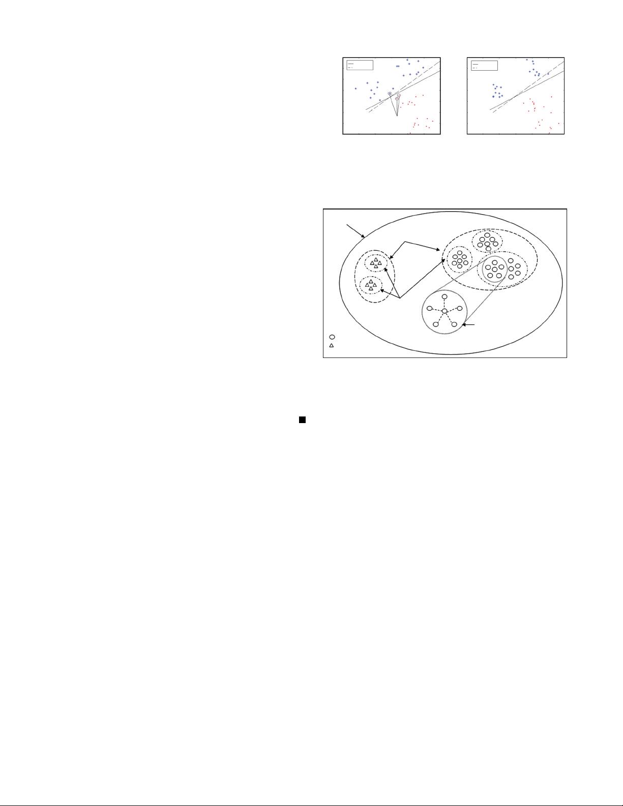
A linear classifier example is illustrated in Fig. 1, where ‘*’
and ‘
.
’ denote the two classes, respectively. Here each class
is generated via a mixture of two Gaussian distributions that
have approximately perpendicular trends of data occurrence.
As we mentioned before, SVM does not sufficiently utilize
the structurally obvious information, and the derived decision
plane, denoted by the dash line in Fig. 1(a), approximately lies
in the middle of three support vectors [4]–[6] in the training
set, which leads to inaccurate classification in the testing set
[Fig. 1(b)]. However, a more reasonable decision plane should
be as denoted by the solid line in Fig. 1. This boundary has
almost parallel orientation to the ‘
.
’ class data trend, and,
at the same time, relatively far from the ‘*’ class due to
the approximately vertical trend of the corresponding data.
Consequently, SRSVM has better classification performance
both in the training and testing sets.
B. Structural Granularity
Definition 1: Given a dataset T =
{
x
i
, y
i
}
n
i=1
.Let
S
1
, S
2
, ··· , S
t
be a partition of T according to some relation
measure, where the partition characterizes the whole data in
3
SRSVM
SVM
Support vectors
SRSVM
SVM
2
1
0
y
−1
−2
−3
−4
3
2
1
0
y
−1
−2
−3
−4
−2
−1
01
x
(a) (b)
x
234
−2 −101234
Fig. 1. Illustration on the importance of the structural information within
classes in SRSVM and SVM. (a) Discriminant boundaries in the training set.
(b) Discriminant boundaries in the testing set.
Global Granularity
global
Class Granularity
class
Cluster Granularity
cluster
Point Granularity
point
Class I
Class II
Fig. 2. Illustration of structural granularity.
the form of some structures such as cluster, and S
1
∪ S
2
∪
···∪ S
t
= T.HereS
i
(i = 1, 2,...,t) is called structural
granularity.
Clearly, structural granularity relies on the different assump-
tions about the actual data structures in real-world problems.
In our viewpoint, it involves four layers, as illustrated in
Fig. 2, where “
◦
”and“
” denote the two classes respectively.
Moreover, the data in the class I “
◦
” are generated by three
Gaussian distributions and the class II “
” are obtained by
two Gaussian distributions.
According to the Gaussian mixture model [20] for a mix-
ture Gaussian distributions, we can characterize the structural
granularity of the training data by ellipsoids (or clusters),
whose centroids (or means) and covariance matrices reflect
the properties of Gaussian distributions. As a result, four
granularity layers can be differentiated:
Global Granularity: The granularity refers to the dataset
T. With this granularity, the whole data are characterized or
enclosed by a single ellipsoid, as shown by the solid line
ellipsoid in Fig. 2, whose centroid μ
global
and covariance
matrix Σ
global
can be obtained by minimizing the volume
of the ellipsoid [9]
min
Σ
global
,μ
global
ln
Σ
global
s.t.
x
i
− μ
global
T
Σ
−1
global
x
i
− μ
global
≤ 1, (8)
Σ
global
≥ 0.
The corresponding classifier, such as EKM, aims to utilize
such global data structure, or more precisely, global data
scatter in its design.


