MATLAB在最优控制问题中的数值解法
版权申诉
50 浏览量
更新于2024-06-14
收藏 1.92MB PDF 举报
"该资源是一本关于使用 MATLAB 解决最优控制问题的PDF文档,主要介绍如何利用 MATLAB 的间接方法来解决这一领域的复杂问题。书中涵盖了最优控制理论的基础,以及随着计算机技术的发展,它在生物系统、通信网络和社会经济系统等多学科应用中的广泛使用。作者强调,越来越多的人需要学习如何数值求解最优控制问题。"
正文:
最优控制理论自四十年前发展以来,已经成为一个成熟的研究领域。随着计算机技术的进步,最优控制在多个学科的应用中扮演了重要角色,例如在生物系统工程、通信网络设计和社会经济政策制定等方面。因此,理解和掌握如何数值求解最优控制问题变得越来越重要。
早期的经典著作如[1],首次系统地介绍了最优控制的理论和许多有趣的实例,包括时间最优、燃料最优以及线性二次调节器(LQR)问题。这些书籍不仅提供了必要的条件,还尽可能给出了明确的解决方案。后来的[2]是一本简洁而优秀的工程实践导向的书籍,它引入了几种迭代算法,使得数值求解问题变得更加可行。
最近的文献[3]则进一步利用 MATLAB 这一强大的数值计算工具来解决最优控制问题。MATLAB 的使用简化了问题求解的过程,使得非专业背景的用户也能更方便地进行计算。在 MATLAB 中,可以利用内置的优化工具箱,如 fmincon、fminunc 等函数,结合动态系统的状态空间模型,来实现对最优控制问题的求解。
对于间接方法,通常涉及到拉格朗日乘子法和庞加莱-贝尔曼方程(Pontryagin's Maximum Principle)。这些方法通过构建哈密顿函数并寻找其最大值来寻找最优控制策略。在 MATLAB 中,可以通过设置适当的约束条件,运用动态规划或直接线性二次型二次规划(LQG)方法来求解这类问题。
此外,书中可能还会涵盖动态规划(Dynamic Programming)的概念,这是解决最优控制问题的一种重要方法,特别是对于离散时间和连续时间的系统。这种方法通过将整个问题分解为一系列子问题,逐个解决以找到全局最优解。
为了实际应用这些方法,读者需要了解如何建立系统的状态方程和性能指标,并能够将这些数学表达式转化为 MATLAB 可以处理的形式。这通常涉及到微分方程的解析或数值积分,以及矩阵运算的知识。
使用 MATLAB 解决最优控制问题的书籍如所描述的那样,旨在提供一个实用的平台,帮助读者理解和应用数值方法解决复杂的控制问题。通过学习,读者不仅可以掌握最优控制的基本理论,还能获得实际编程和调试经验,从而在实际工程或科研项目中有效地应用这些工具。
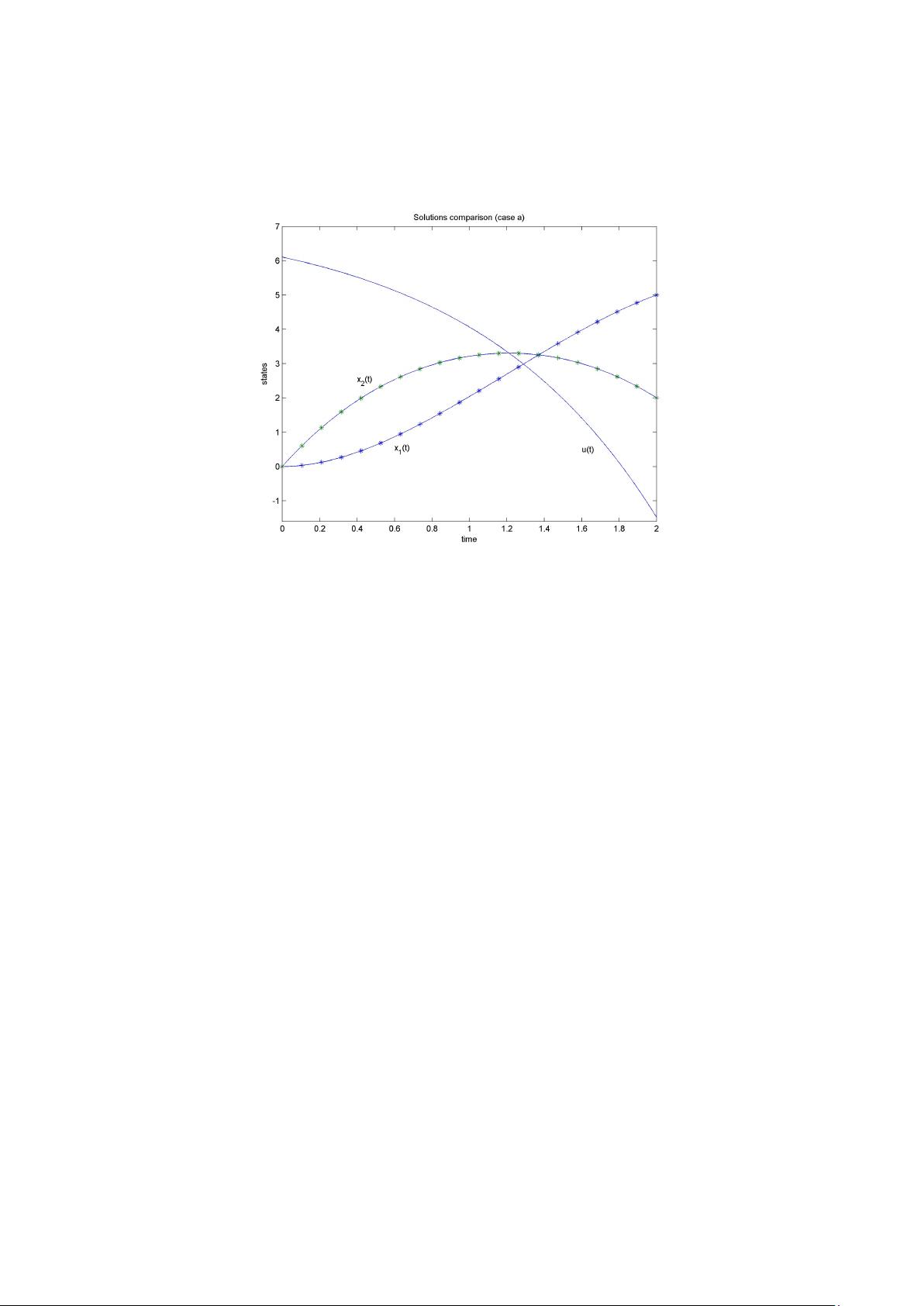
Figure 1: Trajectories for Example 1 (a)
For case (b), we substitute t
0
= 0, t
f
= 2 in the the general solution
to get a set of 4 algebraic equations with 4 arbitrary coefficients. Then
the four boundary conditions are supplied to determine these coefficients.
sol_b is a structure consists of four coefficients returned by solve. We get
the final symbolic solution to the ODE’s by substituting these coefficients
into the general solution. Figure 2 shows the results of both solutions from
MATLAB and [2].
It should be noted that we cannot get the solution by directly supplying
the boundary conditions with dsolve as we did in case (a). Because the
latter two boundary conditions: p
∗
1
(2) = x
∗
1
(t) − 5, p
∗
2
(2) = x
∗
2
(t) − 2 replaces
costates p
1
, p
2
with states x
1
, x
2
in the ODE’s which resulted in more ODE’s
than variables.
% case b: (a) x1(0)=x2(0)=0; p1(2) = x1(2) - 5; p2(2) = x2(2) -2;
eq1b = char(subs(sol_h.x1,’t’,0));
eq2b = char(subs(sol_h.x2,’t’,0));
eq3b = strcat(char(subs(sol_h.p1,’t’,2)),...
’=’,char(subs(sol_h.x1,’t’,2)),’-5’);
eq4b = strcat(char(subs(sol_h.p2,’t’,2)),...
’=’,char(subs(sol_h.x2,’t’,2)),’-2’);
sol_b = solve(eq1b,eq2b,eq3b,eq4b);
5
剩余20页未读,继续阅读
128 浏览量
2021-10-30 上传
2022-10-30 上传
123 浏览量
109 浏览量

百态老人
- 粉丝: 1w+
- 资源: 2万+
 我的内容管理
展开
我的内容管理
展开


最新资源
- ID3算法C语言编写的源程序
- Web Service开发指南
- 基于MC9S12DP256 的电动助力转
- 磁盘阵列详细概述让你彻底明白RAID的各种级别
- 基于DM642的图像处理系统设计及应用.pdf
- QNX安装说明手册。QNX的开发使用
- 2008三级网络技术上机(南开100题)
- 原汁原味的 C# Language Specification 1.2
- siebel工作流管理指南
- JMS简明教程 详细的讲解JMS
- ActiveMQ教程
- WebSphere Service Registry and Repository Handbook
- ORACLE入门心得
- iPhoneAppProgrammingGuide.pdf
- 计算机网络 作业 宝德学院
- tomcat数据源,非常全面.doc
