Dasgupta, Papadimitriou, Vazirani算法专著2008版：理论与实践

5星 · 超过95%的资源需积分: 25 71 浏览量更新于2024-07-25 5 收藏 5.72MB PDF 举报

《算法》(Algorithms)是由Sanjoy Dasgupta、Christos Papadimitriou和Umesh Vazirani三位知名学者合作编写的经典著作，于2008年由McGraw-Hill出版公司发行。本书是计算机科学领域的基石，主要探讨了算法设计与分析的基本原理和实践方法，适用于大学计算机科学课程以及专业人员的深入学习。该书涵盖了广泛的算法主题，包括但不限于排序、搜索、图论、动态规划、贪心算法、递归、复杂性理论等核心内容。作者们以其清晰的阐述、严谨的逻辑和丰富的实例，引导读者理解算法背后的数学思想和工程应用。通过阅读这本书，学生和研究人员能够提升问题解决能力，掌握如何设计高效、优雅的解决方案来处理各种计算问题。书中特别强调了算法分析的重要性，如时间复杂度和空间复杂度的讨论，这些概念对于评估算法效率至关重要。此外，书中的许多章节还探讨了实际编程中的挑战，以及如何将理论转化为实践，特别是在C语言等编程语言中的实现。版权方面，该书受到The McGraw-Hill Companies Inc.的严格保护，未经许可，任何形式的复制、分发或存储都必须得到出版商的书面同意。由于版权限制，某些辅助材料如电子版和打印版可能只在美国境内提供。《算法》不仅是一本教学用书，也是业界专业人士参考的重要资料，它的出版标志着算法研究和教育的一个里程碑。对于想要深入理解算法设计和优化，或是希望在计算机科学领域取得突破的读者来说，这是一本不可或缺的经典教材。无论是在学术研究、工程开发还是日常编程工作中，它都能提供扎实的理论基础和实践经验。

P1: OSO/OVY P2: OSO/OVY QC: OSO/OVY T1: OSO

das23402

Ch00 GTBL020-Dasgupta-v10 August 2, 2006 2:44

Chapter 0 Algorithms

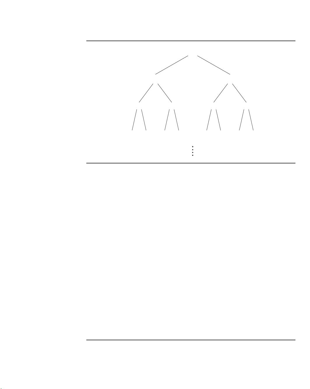
Figure 0.1 The proliferation of recursive calls in fib1.

n−3

n−1

n−4

n−2

n−4

n−6

n−5

n−4

n−2

n−3

n−4

n−5

As with fib1, the correctness of this algorithm is self-evident because it directly

uses the definition of F

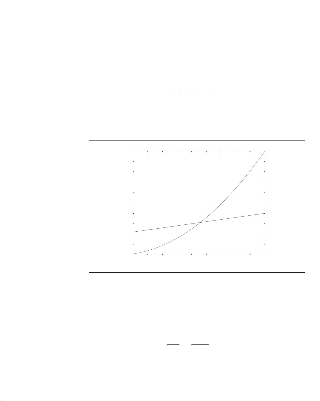
. How long does it take? The inner loop consists of a single

computer step and is executed n − 1 times. Therefore the number of computer steps

used by fib2 is linear in n. From exponential we are down to polynomial, a huge

breakthrough in running time. It is now perfectly reasonable to compute F

200

even F

200,000

As we will see repeatedly throughout this book, the right algorithm makes all the

difference.

More careful analysis

In our discussion so far, we have been counting the number of basic computer steps

executed by each algorithm and thinking of these basic steps as taking a constant

amount of time. This is a very useful simplification. After all, a processor’s instruc-

tion set has a variety of basic primitives—branching, storing to memory, comparing

numbers, simple arithmetic, and so on—and rather than distinguishing between

these elementary operations, it is far more convenient to lump them together into

one category.

But looking back at our treatment of Fibonacci algorithms, we have been too liberal

with what we consider a basic step. It is reasonable to treat addition as a single

computer step if small numbers are being added, 32-bit numbers say. But the nth

Fibonacci number is about 0.694n bits long, and this can far exceed 32 as n grows.

To better appreciate the importance of this dichotomy between exponential and polynomial algorithms,

the reader may want to peek ahead to the story of Sissa and Moore in Chapter 8.

P1: OSO/OVY P2: OSO/OVY QC: OSO/OVY T1: OSO

das23402

Ch00 GTBL020-Dasgupta-v10 August 2, 2006 2:44

6 0.3 Big-O notation

Arithmetic operations on arbitrarily large numbers cannot possibly be performed

in a single, constant-time step. We need to audit our earlier running time estimates

and make them more honest.

We will see in Chapter 1 that the addition of two n-bit numbers takes time roughly

proportional to n; this is not too hard to understand if you think back to the grade-

school procedure for addition, which works on one digit at a time. Thus fib1,

which performs about F

additions, actually uses a number of basic steps roughly

proportional to nF

. Likewise, the number of steps taken by fib2 is proportional

to n

, still polynomial in n and therefore exponentially superior to fib1. This cor-

rection to the running time analysis does not diminish our breakthrough.

But can we do even better than fib2? Indeed we can: see Exercise 0.4.

0.3 Big-O notation

We’ve just seen how sloppiness in the analysis of running times can lead to an

unacceptable level of inaccuracy in the result. But the opposite danger is also

present: it is possible to be too precise. An insightful analysis is based on the right

simplifications.

Expressing running time in terms of basic computer steps is already a simplifica-

tion. After all, the time taken by one such step depends crucially on the particu-

lar processor and even on details such as caching strategy (as a result of which

the running time can differ subtly from one execution to the next). Account-

ing for these architecture-specific minutiae is a nightmarishly complex task and

yields a result that does not generalize from one computer to the next. It there-

fore makes more sense to seek an uncluttered, machine-independent characteriza-

tion of an algorithm’s efficiency. To this end, we will always express running time

by counting the number of basic computer steps, as a function of the size of the

input.

And this simplification leads to another. Instead of reporting that an algorithm takes,

say, 5n

+ 4n + 3 steps on an input of size n, it is much simpler to leave out lower-

order terms such as 4n and 3 (which become insignificant as n grows), and even the

detail of the coefficient 5 in the leading term (computers will be five times faster in

a few years anyway), and just say that the algorithm takes time O(n

) (pronounced

“big oh of n

”).

It is time to define this notation precisely. In what follows, think of f (n) and g(n)

as the running times of two algorithms on inputs of size n.

Let f (n) and g(n) be functions from positive integers to positive reals. We say

f = O(g) (which means that “ f grows no faster than g”) if there is a constant

c > 0 such that f (n) ≤ c · g(n).

Saying f = O (g) is a very loose analog of “ f ≤ g.” It differs from the usual notion

of ≤ because of the constant c, so that for instance 10n = O(n). This constant also

allows us to disregard what happens for small values of n. For example, suppose we

剩余331页未读，继续阅读

craft-zhang

粉丝: 1
资源: 4

Dasgupta, Papadimitriou, Vazirani算法专著2008版：理论与实践

遥感技术详解：植被、土壤判读与应用指南

热红外航空图像：遥感原理与应用深度解析

航空像片判读：步骤、方法与现代遥感应用

algorithms,.s..dasgupta,.c.h..papadimitriou,.u.v..vazirani,.mgh,.2008

遥感图像处理：彩色合成与光学增强

遥感技术与大气环境影响

springboot167基于springboot的医院后台管理系统的设计与实现.zip

XGigE IP GigE Vision Streaming Protocol VHDL源码 有基于AC701 FPGA板卡的完整的参考工程

fluent重叠网格动网格，振荡翼型加摆动后缘小翼算例文件，udf文件，视频教程 流体力学，航空航天，船舶海洋，土木工程，能源动力专业必备

springboot174基于springboot的疾病防控综合系统的设计与实现.zip

最新资源

XGigE IP GigE Vision Streaming Protocol VHDL源码有基于AC701 FPGA板卡的完整的参考工程

fluent重叠网格动网格，振荡翼型加摆动后缘小翼算例文件，udf文件，视频教程流体力学，航空航天，船舶海洋，土木工程，能源动力专业必备