JSPCA: 联合稀疏主成分分析提升分类精度

9 浏览量更新于2024-08-26 收藏 2.59MB PDF 举报

联合稀疏主成分分析（Jointsparse Principal Component Analysis, JSPCA）是一项针对高维数据降维问题的研究论文，旨在提升主成分分析（PCA）算法的鲁棒性。PCA作为常用的数据降维工具，其基本原理是通过线性变换将原始数据映射到新的坐标系中，使得数据在新空间中的方差最大化，从而实现维度减少。然而，现有的PCA变种存在局限性，它们要么不能一致地选择有用的特征，要么对异常值敏感，这在分类任务中可能降低性能。 JSPCA的创新之处在于它结合了稀疏学习的概念，引入了混合范数（即L2,1-norm），这使得模型能够同时考虑数据的稀疏性和结构信息。在JSPCA中，目标是找到一组联合稀疏的主成分，这些成分既能保持数据的主要信息，又能抵抗噪声和异常值的影响。这种方法的优势在于： 1. **一致性特征选择**：通过联合稀疏性约束，JSPCA能够在众多特征中找到那些对于数据降维至关重要的子集，这有助于提高特征选择的稳定性和分类的准确性。 2. **抗干扰能力**：由于对异常值的不敏感性，JSPCA能在存在噪声或离群点的情况下，依然能有效地进行有效的降维，减少了这些异常值对降维结果的负面影响。 3. **高效算法设计**：为了求解JSPCA优化问题，研究者可能需要开发高效的算法策略，如迭代优化方法或者基于分块共轭梯度等技术，来寻找最优的联合稀疏主成分。 4. **应用广泛性**：JSPCA不仅适用于传统的监督学习任务，如分类，还可以扩展到其他领域，如图像处理、信号处理、生物信息学等，因为其在保持数据本质特征的同时，降低了数据的复杂性。这篇论文于2016年1月16日接收，并在经过修订后于同年8月21日接受，最终于8月24日在线发布。关键词包括：维度降低、联合稀疏、L2,1范数。通过JSPCA，研究人员希望能够提供一个更为稳健和高效的降维解决方案，从而在实际应用中提高机器学习模型的性能和稳定性。

(a) to illustrate the learned transformation matrix by SPCA. Note

that each row of the transformation matrix corresponds to an

original feature while each column corresponds to a dimension-

ality of the subspace. For one ﬁxed dimensionality of the subspace,

the feature with zero loading is not selected. For example, the ﬁrst

four features are not selected on the second dimensionality but

they are selected on the remaining subspace dimensionality. Be-

sides, the eighth feature is not selected on the third dimensionality

but it is selected on the remaining subspace dimensionality; the

sixth feature is not selected on the sixth dimensionality but it is

selected on the remaining subspace dimensionality. Since the

feature loadings across all the subspace dimensionality cannot be

ignorable, it still cannot tell us that which features are really

useless as a whole. That is, the useless feature cannot be jointly

excluded by SPCA. Inspired by SPCA, we aim to learn a transfor-

mation matrix with row-sparsity, which is shown in the left sub-

ﬁgure in Fig. 1(a). In this way, the learned transformation matrix

can tell us that the third and seventh features are useless. This is

the reason that why we add

ℓ

2,1

-norm on the transformation

matrix.

On the other hand, considering the largely appearing of outliers

in real-world applications, we utilize

ℓ

2,1

-norm on loss term to

enhance the robustness to outliers. In order to test the robustness

to outliers of JSPCA, 200 points near a straight line are generated

with 20 outliers. Then, we apply PCA and JSPCA to this data set,

respectively. From Fig. 1(b), we can see that PCA is signiﬁcantly

affected while JSPCA is affected much less. This is the reason that

why we add

ℓ

2,1

-norm on loss term.

3.2. Objective function of JSPCA

Considering the outliers appearing in data sets and the con-

sistent selection of features, we propose the following optimiza-

tion formulation:

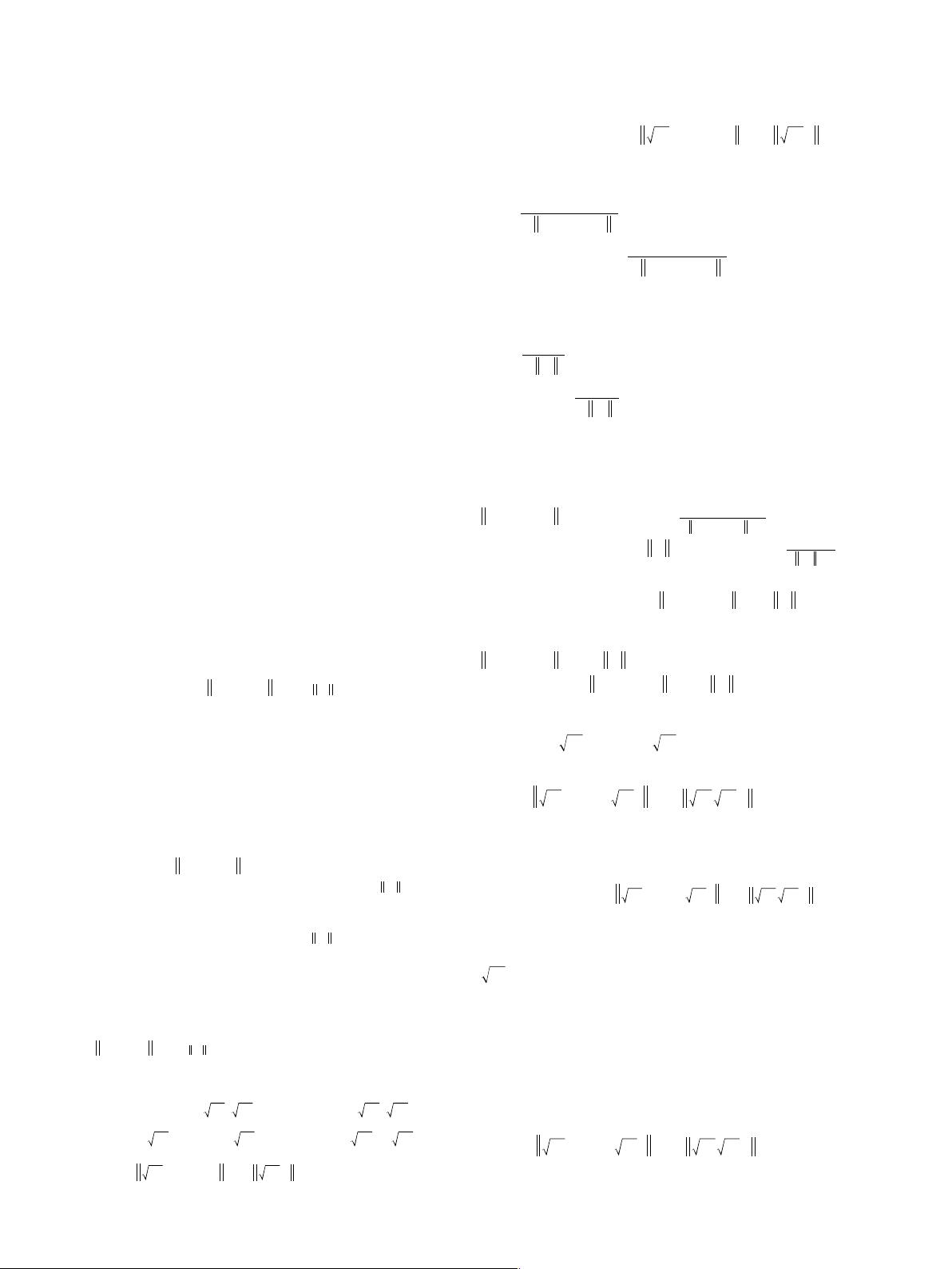
λ()= − +

()

JQ P X PQX Qarg min , arg min ,

QP QP

2,1

where transformation matrix

∈

is ﬁrst used to project the

data matrix X onto a low-dimensional subspace and another

transformation matrix

∈

is then used to recover the data

matrix X. Here, we relax the orthogonal constraint of transfor-

mation matrix Q, introduce another transformation matrix P and

add joint

ℓ

2,1

-norms on both loss term and regularization term. In

this way, JSPCA can have more freedom to learn a low-dimensional

subspace that approximates to high-dimensional data in a ﬂexible

way. The loss term

−XPQX

2,1

is not squared and hence it en-

hances the robustness to outliers. The penalty term

2,1

pena-

lizes all m regression coefﬁcients corresponding to a single feature

as a whole and hence our method is able to jointly select features.

On the other hand, the regularization term

2,1

is convex and can

be easily optimized.

≥

, as a regularization parameter, is used to

balance the loss term and regularization term.

Directly solving Eq. (2) is difﬁcult as both loss term and reg-

ularization term are non-smooth [1]. Using some mathematical

techniques for Eq. (2), we have,

()

−+

=((−)(−))+()

=((−)(−))+( )

= (((−))(−))+(( ) )

=(−)+

XPQX Q

XPQXDXPQX QDQ

XPQX D DXPQX QD DQ

D X PQX D X PQX DQ DQ

DX PQX DQ

arg min

arg min 2tr 2 tr

arg min tr tr

arg min .

TT T T

2,1

11 22

Hence, Eq. (2) becomes,

λ()= (− )+

()

JQ P D X PQX D Qarg min , arg min ,

QP QP

where

(− )

⋱()

⎡

⎣

⎢

⎤

⎦

⎥

XPQX

and

⋱()

⎡

⎣

⎢

⎤

⎦

⎥

are two

×m

diagonal matrices. Note that

(− )XPQX

(= …

)

im1, 2, ,

means the i-th row of matrix

−

, and Q

(= …

)

im1, 2, ,

means the i-th row of matrix Q. When

(− ) =XPQX

, we let

ζ(− ) +

XPQX

(

is a very small

constant). Similarly, when

, we let

ζ+

. In this

way, the smaller the

is, the more important the i-th feature is.

Moreover, we can see that if

(− )XPQX

and

are small, D

and D

are large and thus the minimization of

λ(( − ) ( − )) + (

)

XPQXDXPQX QDQ

tr 2 tr

TT T T

in Eq. (3) tends to force

(− )XPQX

and

to be a very small value. After several

iterations, some

(− )XPQX

and

(= …

)

Qi m1, 2, ,

may be

close to zero and thus we obtain a joint sparse Q and a small re-

construction loss.

Next, let

, and

−

. Then, the formulation in

Eq. (4) can be rewritten as,

λ−

()

¯¯

DX PQ DX D DQarg min .

In order to reduce the feature redundancy, we impose the ortho-

gonal constraint

¯¯

PP I

for Eq. (7). Then, we have,

()

λ(

¯¯

)= −

¯¯

¯¯ ¯¯

JQ P D X PQ D X D D Q

PP I

arg min , arg min ,

s. t. ,

QP QP

where

∈

is ﬁrst used to project the weighted data matrix

and

∈

is then used to recover it.

3.3. The optimal solution

The solution of Eq. (8) is divided into the below two steps:

Step 1: Given

, there exists an optimal matrix

⊥

such that

[

¯¯

]

⊥

PP,

×m

column orthogonal matrix. Then, optimization

problem in Eq. (8) becomes,

λ−

()

DX PQ DX D DQarg min .

The ﬁrst part of Eq. (9) can be rewritten as,

S. Yi et al. / Pattern Recognition 61 (2017) 524–536526

剩余12页未读，继续阅读

weixin_38736652

粉丝: 1
资源: 938

JSPCA: 联合稀疏主成分分析提升分类精度

高光谱图像分类：主成分分析与局部二值模式结合的算法

新型联合稀疏散列法提升图像检索效率

形状自适应联合稀疏表示法提升高光谱图像分类性能

spca:spca 是一个用于稀疏主成分分析的 R 包

基于鲁棒主成分分析的多域联合杂波抑制算法.docx

深度子空间联合稀疏表示单样本人脸识别算法.pdf

联合特征选择的稀疏度保留分数

原子-分子字典结合的联合扩展加权稀疏表示人脸识别算法.pdf

基于人脸识别分类器（SRC）的LBP算法与稀疏表达联合方法的改进

稀疏编码ICCV2009教程

最新资源