没有合适的资源?快使用搜索试试~ 我知道了~
首页Factor Graphs and GTSAM
Factor Graphs and GTSAM
需积分: 50 23 下载量 171 浏览量
更新于2023-03-03
评论
收藏 1.41MB PDF 举报
FactorGraphsandGTSAM 这个是gtsam作者做的一个使用文档,里面详细讲解了如何使用gtsam库,很多例子
资源详情
资源评论
资源推荐
Factor Graphs and GTSAM:
A Hands-on Introduction
Frank Dellaert
Technical Report number GT-RIM-CP&R-2012-002
September 2012
Overview
In this document I provide a hands-on introduction to both factor graphs and GTSAM.
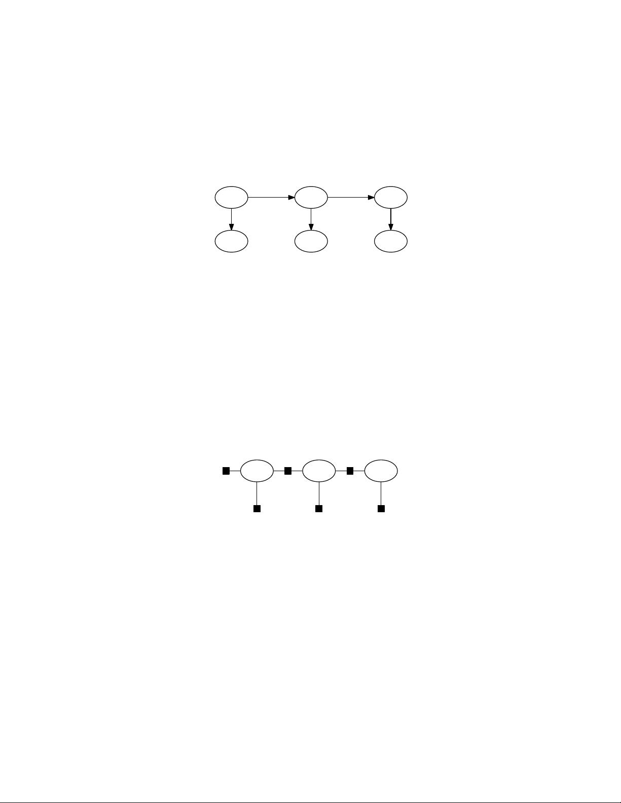
Factor graphs are graphical models (Koller and Friedman, 2009) that are well suited to mod-
eling complex estimation problems, such as Simultaneous Localization and Mapping (SLAM) or
Structure from Motion (SFM). You might be familiar with another often used graphical model,
Bayes networks, which are directed acyclic graphs. A factor graph, however, is a bipartite graph
consisting of factors connected to variables. The variables represent the unknown random vari-
ables in the estimation problem, whereas the factors represent probabilistic information on those
variables, derived from measurements or prior knowledge. In the following sections I will show
many examples from both robotics and vision.
The GTSAM toolbox (GTSAM stands for “Georgia Tech Smoothing and Mapping”) toolbox is
a BSD-licensed C++ library based on factor graphs, developed at the Georgia Institute of Technol-
ogy by myself, many of my students, and collaborators. It provides state of the art solutions to the
SLAM and SFM problems, but can also be used to model and solve both simpler and more com-
plex estimation problems. It also provides a MATLAB interface which allows for rapid prototype
development, visualization, and user interaction.
GTSAM exploits sparsity to be computationally efficient. Typically measurements only provide
information on the relationship between a handful of variables, and hence the resulting factor graph
will be sparsely connected. This is exploited by the algorithms implemented in GTSAM to reduce
computational complexity. Even when graphs are too dense to be handled efficiently by direct
methods, GTSAM provides iterative methods that are quite efficient regardless.
You can download the latest version of GTSAM at http://tinyurl.com/gtsam.
1
Contents
1 Factor Graphs 3
2 Modeling Robot Motion 4
2.1 Modeling with Factor Graphs . . . . . . . . . . . . . . . . . . . . . . . . . . . . . 4
2.2 Creating a Factor Graph . . . . . . . . . . . . . . . . . . . . . . . . . . . . . . . . 4
2.3 Factor Graphs versus Values . . . . . . . . . . . . . . . . . . . . . . . . . . . . . 5
2.4 Non-linear Optimization in GTSAM . . . . . . . . . . . . . . . . . . . . . . . . . 6
2.5 Full Posterior Inference . . . . . . . . . . . . . . . . . . . . . . . . . . . . . . . . 7
3 Robot Localization 8
3.1 Unary Measurement Factors . . . . . . . . . . . . . . . . . . . . . . . . . . . . . 8
3.2 Defining Custom Factors . . . . . . . . . . . . . . . . . . . . . . . . . . . . . . . 8
3.3 Using Custom Factors . . . . . . . . . . . . . . . . . . . . . . . . . . . . . . . . . 10
3.4 Full Posterior Inference . . . . . . . . . . . . . . . . . . . . . . . . . . . . . . . . 10
4 PoseSLAM 12
4.1 Loop Closure Constraints . . . . . . . . . . . . . . . . . . . . . . . . . . . . . . . 12
4.2 Using the MATLAB Interface . . . . . . . . . . . . . . . . . . . . . . . . . . . . 14
4.3 Reading and Optimizing Pose Graphs . . . . . . . . . . . . . . . . . . . . . . . . 15
4.4 PoseSLAM in 3D . . . . . . . . . . . . . . . . . . . . . . . . . . . . . . . . . . . 17
5 Landmark-based SLAM 18
5.1 Basics . . . . . . . . . . . . . . . . . . . . . . . . . . . . . . . . . . . . . . . . . 18
5.2 Of Keys and Symbols . . . . . . . . . . . . . . . . . . . . . . . . . . . . . . . . . 19
5.3 A Larger Example . . . . . . . . . . . . . . . . . . . . . . . . . . . . . . . . . . . 20
5.4 A Real-World Example . . . . . . . . . . . . . . . . . . . . . . . . . . . . . . . . 21
6 Structure from Motion 22
7 More Applications 24
7.1 Conjugate Gradient Optimization . . . . . . . . . . . . . . . . . . . . . . . . . . . 24
7.2 Visual Odometry . . . . . . . . . . . . . . . . . . . . . . . . . . . . . . . . . . . 25
7.3 Visual SLAM . . . . . . . . . . . . . . . . . . . . . . . . . . . . . . . . . . . . . 25
7.4 Fixed-lag Smoothing and Filtering . . . . . . . . . . . . . . . . . . . . . . . . . . 25
7.5 iSAM: Incremental Smoothing and Mapping . . . . . . . . . . . . . . . . . . . . . 25
7.6 Discrete Variables and HMMs . . . . . . . . . . . . . . . . . . . . . . . . . . . . 25
2
1 Factor Graphs
Let us start with a one-page primer on factor graphs, which in no way replaces the excellent and
detailed reviews by Kschischang et al. (2001) and Loeliger (2004).
Figure 1: An HMM, unrolled over three time-steps, represented by a Bayes net.
Figure 1 shows the Bayes network for a hidden Markov model (HMM) over three time steps.
In a Bayes net each node is associated with a conditional density: the top Markov chain encodes
the prior P (X
0
) and transition probabilities P (X
2
|X
1
) and P (X
3
|X
2
), whereas measurements Z
t
depend only on the state X
t
, modeled by conditional densities P (Z
t
|X
t
). Given known measure-
ments z
1
, z
2
and z
3
we are interested in the hidden state sequence (X
1
,X
2
,X
3
) that maximizes the
posterior probability P (X
1
,X
2
,X
3
|Z
1
= z
1
,Z
2
= z
2
,Z
3
= z
3
). Since the measurements Z
1
, Z
2
,
and Z
3
are known, the posterior is proportional to the product of six factors, three of which derive
from the the Markov chain, and three likelihood factors defined as L(X
t
; z) / P (Z
t
= z|X
t
):
P (X
1
,X
2
,X
3
|Z
1
,Z
2
,Z
3
) / P (X
1
)P (X
2
|X
1
)P (X
3
|X
2
)L(X
1
; z
1
)L(X
2
; z
2
)L(X
3
; z
3
)
Figure 2: An HMM with observed measurements, unrolled over time, represented as a factor graph.
This motivates a different graphical model, a factor graph, in which we only represent the un-
known variables X
1
, X
2
, and X
3
, connected to factors that encode probabilistic information on
them, as in Figure 2. To do maximum a-posteriori (MAP) inference, we then maximize the product
f(X
1
,X
2
,X
3
)=
Y
f
i
(X
i
)
i.e., the value of the factor graph. It should be clear from the figure that the connectivity of a factor
graph encodes for each factor f
i
on which subset of variables X
i
it depends. In the examples below,
we use factor graphs to model more complex MAP inference problems in robotics.
3
2 Modeling Robot Motion
2.1 Modeling with Factor Graphs
Before diving into a SLAM example, let us consider the simpler problem of modeling robot motion,
which can be done with a continuous Markov chain, and provides a gentle introduction to GTSAM.
x
1
x
2
x
3
f
0
(x
1
)
f
1
(x
1
,x
2
; o
1
) f
2
(x
2
,x
3
; o
2
)
Figure 3: Factor graph for robot localization.
The factor graph for a simple example is shown in Figure 3. There are three variables x
1
, x
2
,
and x
3
which represent the poses of the robot over time, rendered in the figure by the open-circle
variable nodes. In this example, we have one unary factor f
0
(x
1
) on the first pose x
1
that encodes
our prior knowledge about x
1
, and two binary factors that relate successive poses, respectively
f
1
(x
1
,x
2
; o
1
) and f
2
(x
2
,x
3
; o
2
), where o
1
and o
2
represent odometry measurements.
2.2 Creating a Factor Graph
The following C++ code, included in GTSAM as an example, creates the factor graph in Figure 3:
1 // Create an empty nonlinear factor graph
2 NonlinearFactorGraph graph;
3
4 // Add a Gaussian prior on pose x_1
5 Pose2 priorMean(0.0, 0.0, 0.0);
6 noiseModel::Diagonal::shared_ptr priorNoise =
7 noiseModel::Diagonal::Sigmas(Vector_(3, 0.3, 0.3, 0.1));
8 graph.add(PriorFactor<Pose2>(1, priorMean, priorNoise));
9
10 // Add two odometry factors
11 Pose2 odometry(2.0, 0.0, 0.0);
12 noiseModel::Diagonal::shared_ptr odometryNoise =
13 noiseModel::Diagonal::Sigmas(Vector_(3, 0.2, 0.2, 0.1));
14 graph.add(BetweenFactor<Pose2>(1, 2, odometry, odometryNoise));
15 graph.add(BetweenFactor<Pose2>(2, 3, odometry, odometryNoise));
Listing 1: Excerpt from examples/OdometryExample.cpp
Above, line 2 creates an empty factor graph. We then add the factor f
0
(x
1
) on lines 5-8 as an
instance of PriorFactor<T>, a templated class provided in the slam subfolder, with T=Pose2. Its
4
constructor takes a variable Key (in this case 1), a mean of type Pose2, created on Line 5, and a
noise model for the prior density. We provide a diagonal Gaussian of type noiseModel::Diagonal
by specifying three standard deviations in line 7, respectively 30 cm. on the robot’s position, and
0.1 radians on the robot’s orientation. Note that the Sigmas constructor returns a shared pointer,
anticipating that typically the same noise models are used for many different factors.
Similarly, odometry measurements are specified as Pose2 on line 11, with a slightly different
noise model defined on line 12-13. We then add the two factors f
1
(x
1
,x
2
; o
1
) and f
2
(x
2
,x
3
; o
2
) on
lines 14-15, as instances of yet another templated class, BetweenFactor<T>, again with T=Pose2.
When running the example (make LocalizationExample.run on the command prompt), will
print out the factor graph as follows:
Factor Graph:
size: 3
factor 0: PriorFactor on 1
prior mean: (0, 0, 0)
noise model: diagonal sigmas [0.3; 0.3; 0.1];
factor 1: BetweenFactor(1,2)
measured: (2, 0, 0)
noise model: diagonal sigmas [0.2; 0.2; 0.1];
factor 2: BetweenFactor(2,3)
measured: (2, 0, 0)
noise model: diagonal sigmas [0.2; 0.2; 0.1];
2.3 Factor Graphs versus Values
At this point it is instructive to emphasize two important design ideas underlying GTSAM:
1. The factor graph and its embodiment in code specify the joint probability distribution P (X|Z)
over the entire trajectory X
= {x
1
,x
2
,x
3
} of the robot, rather than just the last pose. This
smoothing view of the world gives GTSAM its name: “smoothing and mapping”. Later in
this document we will talk about how we can also use GTSAM to do filtering (which you
often do not want to do) or incremental inference (which we do all the time).
2. A factor graph in GTSAM is just the specification of the probability density P (X|Z), and
the corresponding C++ FactorGraph and its derived classes do not ever contain a “solution”.
Rather, there is a separate type Values that can be used to specify specific values for (in this
case) x
1
, x
2
, and x
3
, which can then be used to evaluate the probability (or, more commonly,
the error) associated with particular values.
The latter point is often a point of confusion with beginning users of GTSAM. It helps to remember
that when designing GTSAM we took a functional approach of classes corresponding to mathemat-
5
剩余26页未读,继续阅读
yariel
- 粉丝: 8
- 资源: 3
上传资源 快速赚钱
- 我的内容管理 收起
- 我的资源 快来上传第一个资源
- 我的收益 登录查看自己的收益
- 我的积分 登录查看自己的积分
- 我的C币 登录后查看C币余额
- 我的收藏
- 我的下载
- 下载帮助
会员权益专享
最新资源
- c++校园超市商品信息管理系统课程设计说明书(含源代码) (2).pdf
- 建筑供配电系统相关课件.pptx
- 企业管理规章制度及管理模式.doc
- vb打开摄像头.doc
- 云计算-可信计算中认证协议改进方案.pdf
- [详细完整版]单片机编程4.ppt
- c语言常用算法.pdf
- c++经典程序代码大全.pdf
- 单片机数字时钟资料.doc
- 11项目管理前沿1.0.pptx
- 基于ssm的“魅力”繁峙宣传网站的设计与实现论文.doc
- 智慧交通综合解决方案.pptx
- 建筑防潮设计-PowerPointPresentati.pptx
- SPC统计过程控制程序.pptx
- SPC统计方法基础知识.pptx
- MW全能培训汽轮机调节保安系统PPT教学课件.pptx
资源上传下载、课程学习等过程中有任何疑问或建议,欢迎提出宝贵意见哦~我们会及时处理!
点击此处反馈
安全验证
文档复制为VIP权益,开通VIP直接复制
信息提交成功
评论0