自监督学习：生成和对比方法综述_自监督学习

自监督学习

需积分: 50 2.9k 浏览量更新于2023-05-27 评论 1 收藏 7.47MB PDF 举报

身份认证购VIP最低享 7 折!

领优惠券(最高得80元）

资源详情

资源评论

资源推荐

Self-supervised Learning: Generative or Contrastive

Xiao Liu, Fanjin Zhang, Zhenyu Hou, Li Mian, Zhaoyu Wang, Jing Zhang, Jie Tang, Senior Member

Abstract

—Deep supervised learning has achieved great success in the last decade. However, its deﬁciencies of dependence on manual

labels and vulnerability to attacks have driven people to explore a better solution. As an alternative, self-supervised learning attracts many

researchers for its soaring performance on representation learning in the last several years. Self-supervised representation learning

leverages input data itself as supervision and beneﬁts almost all types of downstream tasks. In this survey, we take a look into new

self-supervised learning methods for representation in computer vision, natural language processing, and graph learning. We

comprehensively review the existing empirical methods and summarize them into three main categories according to their objectives:

generative, contrastive, and generative-contrastive (adversarial). We further investigate related theoretical analysis work to provide

deeper thoughts on how self-supervised learning works. Finally, we brieﬂy discuss open problems and future directions for

self-supervised learning.

Index Terms—Self-supervised Learning, Generative Model, Contrastive Learning, Deep Learning

1 INTRODUCTION

eep neural networks [77] have shown outstanding

performance on various machine learning tasks, es-

pecially on supervised learning in computer vision (image

classiﬁcation [32], [54], [59], semantic segmentation [45],

[85]), natural language processing (pre-trained language

models [33], [74], [84], [149], sentiment analysis [83], question

answering [5], [35], [111], [150] etc.) and graph learning (node

classiﬁcation [58], [70], [106], [138], graph classiﬁcation [7],

[123], [155] etc.). Generally, the supervised learning is trained

over a speciﬁc task with a large manually labeled dataset

which is randomly divided into training, validatiton and test

sets.

However, supervised learning is meeting its bottleneck.

It not only relies heavily on expensive manual labeling

but also suffers from generalization error, spurious cor-

relations, and adversarial attacks. We expect the neural

network to learn more with fewer labels, fewer samples,

or fewer trials. As a promising candidate, self-supervised

learning has drawn massive attention for its fantastic data

efﬁciency and generalization ability, with many state-of-

the-art models following this paradigm. In this survey, we

will take a comprehensive look at the development of the

recent self-supervised learning models and discuss their

theoretical soundness, including frameworks such as Pre-

trained Language Models (PTM), Generative Adversarial

•

Xiao Liu, Fanjin Zhang, and Zhengyu Hou are with the Department of

Computer Science and Technology, Tsinghua University, Beijing, China.

E-mail: liuxiao17@mails.tsinghua.edu.cn, zfj17@mails.tsinghua.edu.cn,

hzy17@mails.tsinghua.edu.cn

•

Jie Tang is with the Department of Computer Science and Technology,

Tsinghua University, and Tsinghua National Laboratory for Information

Science and Technology (TNList), Beijing, China, 100084.

E-mail: jietang@tsinghua.edu.cn, corresponding author

• Li Mian is with the Beijing Institute of Technonlogy, Beijing, China.

Email: 1120161659@bit.edu.cn

• Zhaoyu Wang is with the Anhui University, Anhui, China.

Email: wzy950507@163.com

• Jing Zhang is with the Renming University of China, Beijing, China.

Email: zhang-jing@ruc.edu.cn

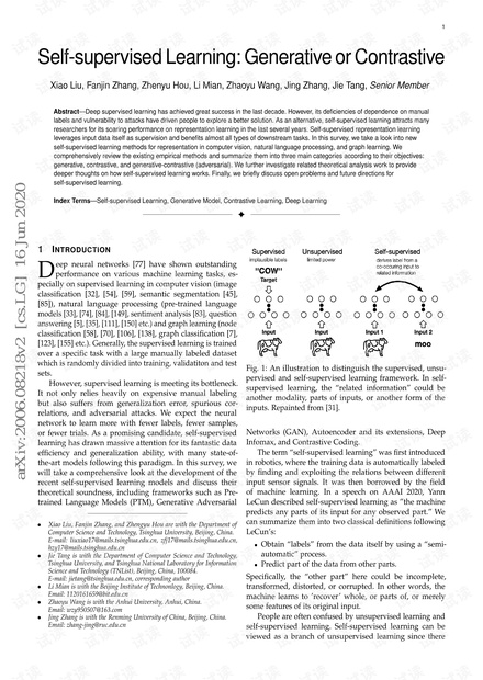
Fig. 1: An illustration to distinguish the supervised, unsu-

pervised and self-supervised learning framework. In self-

supervised learning, the “related information” could be

another modality, parts of inputs, or another form of the

inputs. Repainted from [31].

Networks (GAN), Autoencoder and its extensions, Deep

Infomax, and Contrastive Coding.

The term “self-supervised learning” was ﬁrst introduced

in robotics, where the training data is automatically labeled

by ﬁnding and exploiting the relations between different

input sensor signals. It was then borrowed by the ﬁeld

of machine learning. In a speech on AAAI 2020, Yann

LeCun described self-supervised learning as ”the machine

predicts any parts of its input for any observed part.” We

can summarize them into two classical deﬁnitions following

LeCun’s:

•

Obtain “labels” from the data itself by using a “semi-

automatic” process.

• Predict part of the data from other parts.

Speciﬁcally, the “other part” here could be incomplete,

transformed, distorted, or corrupted. In other words, the

machine learns to ’recover’ whole, or parts of, or merely

some features of its original input.

People are often confused by unsupervised learning and

self-supervised learning. Self-supervised learning can be

viewed as a branch of unsupervised learning since there

arXiv:2006.08218v2 [cs.LG] 16 Jun 2020

is no manual label involved. However, narrowly speaking,

unsupervised learning concentrates on detecting speciﬁc

data patterns, such as clustering, community discovery, or

anomaly detection, while self-supervised learning aims at

recovering, which is still in the paradigm of supervised set-

tings. Figure 1 provides a vivid explanation of the differences

between them.

There exist several comprehensive reviews related to Pre-

trained Language Models [107], Generative Adversarial Net-

works [142], Autoencoder and contrastive learning for visual

representation [64]. However, none of them concentrates on

the inspiring idea of self-supervised learning that illustrates

researchers and models in many ﬁelds. In this work, we

collect studies from natural language processing, computer

vision, and graph learning in recent years to present an up-

to-date and comprehensive retrospective on the frontier of

self-supervised learning. To sum up, our contributions are:

•

We provide a detailed and up-to-date review of self-

supervised learning for representation. We introduce

the background knowledge, models with variants, and

important frameworks. One can easily grasp the frontier

ideas of self-supervised learning.

•

We categorize self-supervised learning models into

generative, contrastive, and generative-contrastive (ad-

versarial), with particular genres inner each one. We

demonstrate the pros and cons of each category and

discuss the recent attempt to shift from generative to

contrastive.

•

We examine the theoretical soundness of self-supervised

learning methods and show how it can beneﬁt the

downstream supervised learning tasks.

•

We identify several open problems in this ﬁeld, analyze

the limitations and boundaries, and discuss the future

direction for self-supervised representation learning.

We organize the survey as follows. In Section 2, we

introduce the preliminary knowledge for new computer

vision, natural language processing, and graph learning.

From Section 3 to Section 5, we will introduce the empirical

self-supervised learning methods utilizing generative, con-

trastive and generative-contrastive objectives. In Section 6,

we investigate the theoretical basis behind the success of self-

supervised learning and its merits and drawbacks. In Section

7, we discuss the open problems and future directions in this

ﬁeld.

2 B ACKGROUND

2.1 Representation Learning in NLP

Pre-trained word representations are key components in

natural language processing tasks. Word embedding is to

represent words as low-dimensional real-valued vectors.

There are two kinds of word embeddings: non-contextual

and contextual embeddings.

Non-contextual Embeddings does not consider the con-

text information of the token; that is, these models only

map the token into a distributed embedding space. Thus, for

each word

in the vocabulary

, embedding will assign

it a speciﬁc vector.

∈ R

, where

is the dimension of

the embedding. These embeddings can not model complex

characteristics of word use and polysemous.

Fig. 2: Number of publications and citations on self-

supervised learning from 2012-2019. Self-supervised learning

is gaining huge attention in recent years. Data from Microsoft

Academic Graph [121]. This only includes paper containing

the complete keyword “self-supervised learning”, so the real

number should be even larger.

To model both complex characteristics of word use and

polysemy, contextual embedding is proposed. For a text

sequence

, x

, ..., x

∈ V

, the contextual embedding

of x

depends on the whole sequence.

, e

, ..., e

] = f(x

, x

, ..., x

here

f(·)

is the embedding function. Since for a certain token

, the embedding

can be different if

in difference

context,

is called contextual embedding. This kind of em-

bedding can distinguish the semantics of words in different

contexts.

Distributed word representation represents each word

as dense, real-valued, and low-dimensional vector. First-

generation word embedding is introduced as a neural

network language model (NNLM) [10]. For NNLM, most

of the complexity is caused by the non-linear hidden layer

in the model. Mikolov et al. proposed Word2Vec Model

[88] [89] to learn the word representations efﬁciently. There

are two models: Continuous Bag-of-Words Model (CBOW)

and Continuous Skip-gram Model (SG). Word2Vec is a

kind of context prediction model, and it is one of the

most popular implementations to generate non-contextual

word embeddings for NLP. In the ﬁrst-generation word

embedding, the same word has the same embedding. Since a

word can have multiple senses, therefore, second-generation

word embedding method is proposed. In that case, each

word token has its embedding. These embeddings also called

contextualized word embedding since the embeddings of

word tokens depend on its context. ELMo (Embeddings from

Language Model) [102] is one implementation to generate

those contextual word embeddings. ELMo is an RNN-based

bidirectional language model, it learns multiple embedding

for each word token, and dependent on how to combine

those embeddings based on the downstream tasks. ELMo

is a feature-based approach, that is, the model is used as a

feature extractor to extract word embedding, and send those

embeddings to the downstream task model. The parameters

of the extractor are ﬁxed, only the parameters in the backend

model can be trained.

Recently, BERT (Bidirectional Encoder Representations

from Transformers) [33] bring large improvements on 11

NLP tasks. Different from feature-based approaches like

ELMo, BERT is a ﬁne-tuned approach. The model is ﬁrst pre-

trained on a large number of corpora through self-supervised

learning, then ﬁne-tuned with labeled data. As the name

showed, BERT is an encoder of the transformer, in the

training stage, BERT masked some tokens in the sentence,

then training to predict the masked word. When use BERT,

initialized the BERT model with pre-trained weights, and

ﬁne-tune the pre-trained model to solve downstream tasks.

2.2 Representation Learning in CV

Computer vision is one of the greatest beneﬁted ﬁelds thanks

to deep learning. In the past few years, researchers have

developed a range of efﬁcient network architectures for

supervised tasks. For self-supervised tasks, many of them are

also proved to be useful. In this section, we introduce ResNet

architecture [54], which is the backbone of a large part of the

self-supervised techniques for visual representation models.

Since AlexNet [73], CNN architecture is going deeper and

deeper. While AlexNet had only ﬁve convolutional layers,

the VGG network [120]and GoogleNet (also codenamed

Inception v1) [127] had 19 and 22 layers respectively.

Evidence [120], [127] reveals that network depth is of

crucial importance, and driven by its signiﬁcance of depth,

a question arises: Is learning better networks as easy as

stacking more layers? An obstacle to answering this question

was the notorious problem of vanishing/exploding gradients

[12], which hamper convergence from the beginning. This

problem, however, has been addressed mainly by normal-

ized initialization [79], [116]and intermediate normalization

layers [61], which enable networks with tens of layers to

start converging for stochastic gradient descent (SGD) with

backpropagation [78].

When deeper networks can start converging, a degra-

dation problem has been exposed: with the network depth

increasing, accuracy becomes saturated (which might be

unsurprising) and then degrades rapidly. Unexpectedly, such

degradation is not caused by overﬁtting, and adding more

layers to a suitably deep model will lead to higher training

error

Residual neural network (ResNet), proposed by He et al.

[54], effectively resolved this problem. Instead of asking every

few stacked layers to directly learn a desired underlying

mapping, authors of [54] design a residual mapping architec-

ture ResNet. The core idea of ResNet is the introduction of

shortcut connections(Fig. 2), which are those skipping over

one or more layers.

A building block is deﬁned as:

y = F (x, {W

}) + x. (1)

Here

and

are the input and output vectors of the

layers considered. The function

F (x, {W

})

represents the

residual mapping to be learned. For the example in Fig. 2 that

has two layers,

F = W

σ(W

in which

denotes ReLU

[91] and the biases are omitted for simplifying notations. The

operation

F + x

is performed by a shortcut connection and

element-wise addition.

Because of its compelling results, ResNet blew peoples

minds and quickly became one of the most popular ar-

chitectures in various computer vision tasks. Since then,

ResNet architecture has been drawing extensive attention

from researchers, and multiple variants based on ResNet

are proposed, including ResNeXt [145], Densely Connected

CNN [59], wide residual networks [153].

2.3 Representation Learning on Graphs

As a ubiquitous data structure, graphs are extensively

employed in multitudes of ﬁelds and become the backbone

of many systems. The central problem in machine learning

on graphs is to ﬁnd a way to represent graph structure so that

it can be easily utilized by machine learning models [51]. To

tackle this problem, researchers propose a series of methods

for graph representation learning at node level and graph

level, which has become a research spotlight recently.

We ﬁrst deﬁne several basic terminologies. Generally, a

graph is deﬁned as

G = (V, E, X)

, where

denotes a set

of vertices,

|V |

denotes the number of vertices in the graph,

and

E ⊆ (V × V )

denotes a set of edges connecting the

vertices.

X ∈ R

|V |×d

is the optional original vertex feature

matrix. When input features are unavailable,

is set as

orthogonal matrix or initialized with normal distribution,

etc., in order to make the input node features less correlated.

The problem of node representation learning is to learn latent

node representations

Z ∈ R

|V |×d

, which is also termed

as network representation learning, network embedding,

etc. There are also some graph-level representation learning

problems, which aims to learn an embedding for the whole

graph.

In general, existing network embedding approaches are

broadly categorized as (1) factorization-based approaches

such as NetMF [104], [105], GraRep [18], HOPE [97], (2)

shallow embedding approaches such as DeepWalk [101],

LINE [128], HARP [21], and (3) neural network approaches

[19], [82]. Recently, graph convolutional network (GCN)

[70] and its multiple variants have become the dominant

approaches in graph modeling, thanks to the utilization of

graph convolution that effectively fuses graph topology and

node features.

However, the majority of advanced graph representation

learning methods require external guidance like annotated

labels. Many researchers endeavor to propose unsupervised

algorithms [48], [52], [139], which do not rely on any external

labels. Self-supervised learning also opens up an opportunity

for effective utilization of the abundant unlabeled data [99],

[125].

3 GENERATIVE SELF-SUPERVISED LEARNING

3.1 Auto-regressive (AR) Model

Auto-regressive (AR) models can be viewed as “Bayes net

structure” (directed graph model). The joint distribution can

be factorized as a product of conditionals

max

(x) =

t=1

log p

1:t−1

) (2)

where the probability of each variable is dependent on the

previous variables.

Model FOS Type Generator Self-supervision Pretext Task

Hard

NS strategy

GPT/GPT-2 [109], [110] NLP G AR Following words Next word prediction - - -

PixelCNN [134], [136] CV G AR Following pixels Next pixel prediction - - -

NICE [36] CV G

Flow

based

Whole image Image reconstruction

- - -

RealNVP [37] CV G - - -

Glow [68] CV G - - -

word2vec [88], [89] NLP G AE

Context words

CBOW & SkipGram × × End-to-end

FastText [15] NLP G AE CBOW × × End-to-end

DeepWalk-based

[47], [101], [128]

Graph G AE

Graph edges Link prediction

× × End-to-end

VGAE [71] Graph G AE × × End-to-end

BERT [33] NLP G AE

Masked words

Sentence topic

Masked language model,

Next senetence prediction

- - -

SpanBERT [65] NLP G AE Masked words Masked language model - - -

ALBERT [74] NLP G AE

Masked words

Sentence order

Masked language model,

Sentence order prediction

- - -

ERNIE [126] NLP G AE

Masked words

Sentence topic

Masked language model,

Next senetence prediction

- - -

VQ-VAE 2 [112] CV G AE Whole image Image reconstruction - - -

XLNet [149] NLP G AE+AR Masked words Permutation language model - - -

RelativePosition [38] CV C -

Spatial relations

(Context-Instance)

Relative postion prediction - - -

CDJP [67] CV C -

Jigsaw + Inpainting

+ Colorization

× × End-to-end

PIRL [90] CV C - Jigsaw × X Memory bank

RotNet [44] CV C - Rotation Prediction - - -

Deep InfoMax [55] CV C -

Belonging

(Context-Instance)

MI Maximization

× × End-to-end

AMDIM [6] CV C - × X End-to-end

CPC [96] CV C - × × End-to-end

InfoWord [72] NLP C - × × End-to-end

DGI [139] Graph C - X × End-to-end

InfoGraph [123] Graph C - × ×

End-to-end

(batch-wise)

GRL [99] Graph C - × × End-to-end

Pre-trained GNN [57] Graph C -

Belonging

Node attributes

MI maximization,

Masked attribute prediction

× × End-to-end

DeepCluster [20] CV C -

Similarity

(Context-Context)

Cluster discrimination

- - -

Local Aggregation [160] CV C - - - -

ClusterFit [147] CV C - - - -

InstDisc [144] CV C -

Identity

(Context-Context)

Instance discrimination

× × Memory bank

CMC [130] CV C - × X End-to-end

MoCo [53] CV C - × × Momentum

MoCo v2 [25] CV C - × X Momentum

SimCLR [22] CV C - × X

End-to-end

(batch-wise)

GCC [63] Graph C - × X Momentum

GAN [46] CV G-C AE

Whole image Image reconstruction

- - -

Adversarial AE [86] CV G-C AE - - -

BiGAN/ALI [39], [42] CV G-C AE - - -

BigBiGAN [40] CV G-C AE - - -

Colorization [75] CV G-C AE Image color Colorization - - -

Inpainting [98] CV G-C AE Parts of images Inpainting - - -

Super-resolution [80] CV G-C AE Details of images Super-resolution - - -

ELECTRA [27] NLP G-C AE Masked words Replaced token detection X × End-to-end

WKLM [146] NLP G-C AE Masked entities Replaced entity detection X × End-to-end

ANE [29] Graph G-C AE

Graph edges Link prediction

- - -

GraphGAN [140] Graph G-C AE - - -

GraphSGAN [34] Graph G-C AE Graph nodes Node classiﬁcation - - -

TABLE 1: An overview of recent self-supervised representation learning. For acronyms used, “FOS” refers to ﬁelds of study;

“NS” refers to negative samples; “PS” refers to positive samples; “MI” refers to mutual information. For alphabets in “Type”:

G Generative ; C Contrastive; G-C Generative-Contrastive (Adversarial).

In NLP, the objective of auto-regressive language model-

ing is usually maximizing the likelihood under the forward

autoregressive factorization [149]. GPT [109] and GPT-2 [110]

use Transformer decoder architecture [137] for language

model. Different from GPT, GPT-2 removes the ﬁne-tuning

processes of different tasks. In order to learn uniﬁed represen-

tations that generalize across different tasks, GPT-2 models

p(output|input, task)

, which means given different tasks,

the same inputs can have different outputs.

The auto-regressive models have also been employed

in computer vision, such as PixelRNN [136] and Pixel-

CNN [134]. The general idea is to use auto-regressive

剩余19页未读，继续阅读

syp_net

粉丝: 147
资源: 1197

会员权益专享

自监督学习：生成和对比方法综述

评论0

会员权益专享

最新资源

自监督学习：生成和对比方法综述

评论0

半监督学习都有哪些常用方法？

半监督目标检测的综述

为一篇基于深度学习的超材料结构设计的硕士毕业论文创建一个大纲，这篇论文的创新点是通过深度学习的方法逆向生成二维超材料结构，并对生成的结构进行频域分析，时域分析和案例分析

生成一篇深度学习配准综述

代码生成器:mybatis-plus-generator自定义模板生成 dto、vo、convertor

自监督学习的相关工作整理

为什么不继续生成文献综述了

深度生成对抗网络pytorch

半监督学习的数据集也是由图片与标签文件组成的吗？那这样与监督学习有什么区别？无监督学习是否表示数据集中不需要标签文件只需要图片文件输入即可？

对于复杂的肾脏超声图像分割问题，使用基于unet的全监督学习效果好还是半监督或者无监督学习效果好？github上不同unet开源代码有什么不同？

请给出以下matlab的代码：生成并绘制 NRZ 和 RZ 信号的时域和频域信息

目前有哪些半监督目标检测模型

、利用numpy工具生成一段序列x(例如:linspace()方法可以生成指定范围内的等差数列

你知道什么是自监督学习吗

Lombok的常用注解

成功实现WinXPWin8双系统及不影响Win8系统秒开功能.pdf

ASP电子商务网站建设(源代码+论文).zip

软件设计说明书复习进程.pdf

国产芯片SWM34SVET6-LQFP100封装单片机开发板ALTIUM设计硬件原理图+PCB文件.zip

会员权益专享

最新资源