没有合适的资源?快使用搜索试试~ 我知道了~
首页mplus 8 用户手册 Chapter10 多层次混合建模视图示例.pdf
mplus 8 用户手册 Chapter10 多层次混合建模视图示例.pdf
需积分: 31 9 下载量 72 浏览量
更新于2023-03-03
评论
收藏 329KB PDF 举报
以下是版本 8 Mplus 用户指南的摘录。第 3 章 - 第 13 章包括 250 多个示例。这些示例还包含在 Mplus DVD 上以及生成数据的相应蒙特卡罗模拟设置中。 第一章:导言 第 2 章:开始使用 Mplus 第 3 章:回归和路径分析视图示例 第四章:探索性因素分析视图示例 第五章:确认因子分析和结构方程建模视图示例 第 6 章:生长建模、生存分析和 N=1 时间序列分析视图示例 第 7 章:具有横截面数据视图示例的混合建模 第 8 章:采用纵向数据视图示例的混合建模 第 9 章:具有复杂调查数据视图示例的多层建模 第10章:多层次混合建模视图示例 第11章:缺少数据建模和贝叶斯估计视图示例 第12章:蒙特卡洛模拟研究查看示例 第13章:示例:特殊功能 第14章:特殊建模问题 第 15 章:标题、数据、变量和定义命令 第16章:分析命令 第17章:MODEL命令 第 18 章:输出、保存数据和绘图命令 第19章:蒙特卡洛命令 第20章:Mplus语言摘要 引用/索引
资源详情
资源评论
资源推荐
Examples: Multilevel Mixture Modeling
395
CHAPTER 10
EXAMPLES: MULTILEVEL
MIXTURE MODELING
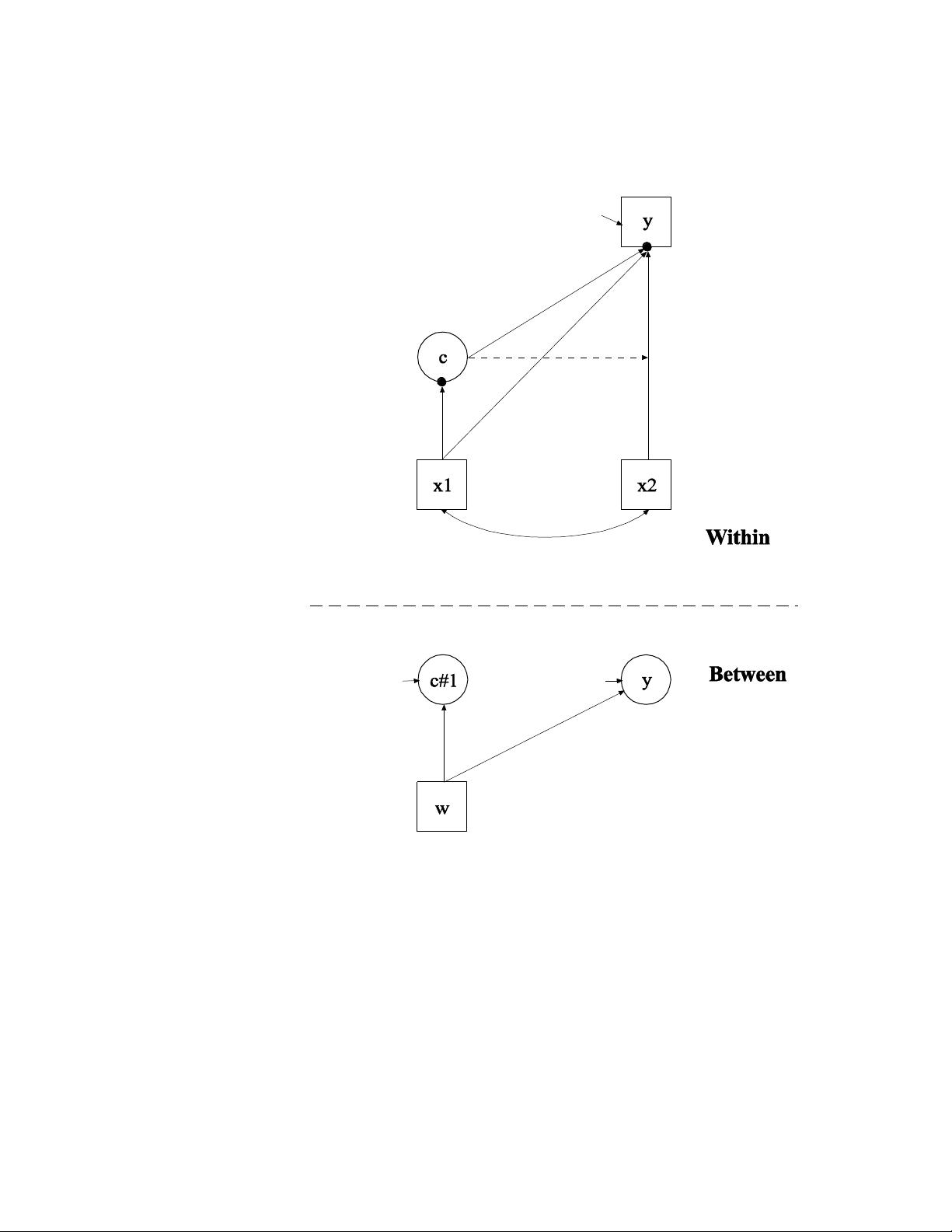
Multilevel mixture modeling (Asparouhov & Muthén, 2008a) combines
the multilevel and mixture models by allowing not only the modeling of
multilevel data but also the modeling of subpopulations where
population membership is not known but is inferred from the data.
Mixture modeling can be combined with the multilevel analyses
discussed in Chapter 9. Observed outcome variables can be continuous,
censored, binary, ordered categorical (ordinal), unordered categorical
(nominal), counts, or combinations of these variable types.
With cross-sectional data, the number of levels in Mplus is the same as
the number of levels in conventional multilevel modeling programs.
Mplus allows two-level modeling. With longitudinal data, the number of
levels in Mplus is one less than the number of levels in conventional
multilevel modeling programs because Mplus takes a multivariate
approach to repeated measures analysis. Longitudinal models are two-
level models in conventional multilevel programs, whereas they are one-
level models in Mplus. Single-level longitudinal models are discussed in
Chapter 6, and single-level longitudinal mixture models are discussed in
Chapter 8. Three-level longitudinal analysis where time is the first level,
individual is the second level, and cluster is the third level is handled by
two-level growth modeling in Mplus as discussed in Chapter 9.
Multilevel mixture models can include regression analysis, path analysis,
confirmatory factor analysis (CFA), item response theory (IRT) analysis,
structural equation modeling (SEM), latent class analysis (LCA), latent
transition analysis (LTA), latent class growth analysis (LCGA), growth
mixture modeling (GMM), discrete-time survival analysis, continuous-
time survival analysis, and combinations of these models.
All multilevel mixture models can be estimated using the following
special features:
Single or multiple group analysis
Missing data
CHAPTER 10
396
Complex survey data
Latent variable interactions and non-linear factor analysis using
maximum likelihood
Random slopes
Individually-varying times of observations
Linear and non-linear parameter constraints
Maximum likelihood estimation for all outcome types
Wald chi-square test of parameter equalities
Analysis with between-level categorical latent variables
Test of equality of means across latent classes using posterior
probability-based multiple imputations
For TYPE=MIXTURE, multiple group analysis is specified by using the
KNOWNCLASS option of the VARIABLE command. The default is to
estimate the model under missing data theory using all available data.
The LISTWISE option of the DATA command can be used to delete all
observations from the analysis that have missing values on one or more
of the analysis variables. Corrections to the standard errors and chi-
square test of model fit that take into account stratification, non-
independence of observations, and unequal probability of selection are
obtained by using the TYPE=COMPLEX option of the ANALYSIS
command in conjunction with the STRATIFICATION, CLUSTER,
WEIGHT, WTSCALE, BWEIGHT, and BWTSCALE options of the
VARIABLE command. Latent variable interactions are specified by
using the | symbol of the MODEL command in conjunction with the
XWITH option of the MODEL command. Random slopes are specified
by using the | symbol of the MODEL command in conjunction with the
ON option of the MODEL command. Individually-varying times of
observations are specified by using the | symbol of the MODEL
command in conjunction with the AT option of the MODEL command
and the TSCORES option of the VARIABLE command. Linear and
non-linear parameter constraints are specified by using the MODEL
CONSTRAINT command. Maximum likelihood estimation is specified
by using the ESTIMATOR option of the ANALYSIS command. The
MODEL TEST command is used to test linear restrictions on the
parameters in the MODEL and MODEL CONSTRAINT commands
using the Wald chi-square test. Between-level categorical latent
variables are specified using the CLASSES and BETWEEN options of
the VARIABLE command. The AUXILIARY option is used to test the
equality of means across latent classes using posterior probability-based
multiple imputations.
Examples: Multilevel Mixture Modeling
397
Graphical displays of observed data and analysis results can be obtained
using the PLOT command in conjunction with a post-processing
graphics module. The PLOT command provides histograms,
scatterplots, plots of individual observed and estimated values, and plots
of sample and estimated means and proportions/probabilities. These are
available for the total sample, by group, by class, and adjusted for
covariates. The PLOT command includes a display showing a set of
descriptive statistics for each variable. The graphical displays can be
edited and exported as a DIB, EMF, or JPEG file. In addition, the data
for each graphical display can be saved in an external file for use by
another graphics program.
Following is the set of cross-sectional examples included in this chapter:
10.1: Two-level mixture regression for a continuous dependent
variable*
10.2: Two-level mixture regression for a continuous dependent
variable with a between-level categorical latent variable*
10.3: Two-level mixture regression for a continuous dependent
variable with between-level categorical latent class indicators for a
between-level categorical latent variable*
10.4: Two-level CFA mixture model with continuous factor
indicators*
10.5: Two-level IRT mixture analysis with binary factor indicators
and a between-level categorical latent variable*
10.6: Two-level LCA with categorical latent class indicators with
covariates*
10.7: Two-level LCA with categorical latent class indicators and a
between-level categorical latent variable
Following is the set of longitudinal examples included in this chapter:
10.8: Two-level growth model for a continuous outcome (three-
level analysis) with a between-level categorical latent variable*
10.9: Two-level GMM for a continuous outcome (three-level
analysis)*
10.10: Two-level GMM for a continuous outcome (three-level
analysis) with a between-level categorical latent variable*
10.11: Two-level LCGA for a three-category outcome*
10.12: Two-level LTA with a covariate*
CHAPTER 10
398
10.13: Two-level LTA with a covariate and a between-level
categorical latent variable
* Example uses numerical integration in the estimation of the model.
This can be computationally demanding depending on the size of the
problem.
EXAMPLE 10.1: TWO-LEVEL MIXTURE REGRESSION FOR
A CONTINUOUS DEPENDENT VARIABLE
TITLE: this is an example of a two-level mixture
regression for a continuous dependent
variable
DATA: FILE IS ex10.1.dat;
VARIABLE: NAMES ARE y x1 x2 w class clus;
USEVARIABLES = y x1 x2 w;
CLASSES = c (2);
WITHIN = x1 x2;
BETWEEN = w;
CLUSTER = clus;
ANALYSIS: TYPE = TWOLEVEL MIXTURE;
STARTS = 0;
MODEL:
%WITHIN%
%OVERALL%
y ON x1 x2;
c ON x1;
%c#1%
y ON x2;
y;
%BETWEEN%
%OVERALL%
y ON w;
c#1 ON w;
c#1*1;
%c#1%
[y*2];
OUTPUT: TECH1 TECH8;
Examples: Multilevel Mixture Modeling
399
In this example, the two-level mixture regression model for a continuous
dependent variable shown in the picture above is estimated. This
example is the same as Example 7.1 except that it has been extended to
the multilevel framework. In the within part of the model, the filled
circles at the end of the arrows from x1 to c and y represent random
intercepts that are referred to as c#1 and y in the between part of the
model. In the between part of the model, the random intercepts are
shown in circles because they are continuous latent variables that vary
剩余47页未读,继续阅读
jlzhangyi
- 粉丝: 6
- 资源: 55
上传资源 快速赚钱
- 我的内容管理 收起
- 我的资源 快来上传第一个资源
- 我的收益 登录查看自己的收益
- 我的积分 登录查看自己的积分
- 我的C币 登录后查看C币余额
- 我的收藏
- 我的下载
- 下载帮助
会员权益专享
最新资源
- RTL8188FU-Linux-v5.7.4.2-36687.20200602.tar(20765).gz
- c++校园超市商品信息管理系统课程设计说明书(含源代码) (2).pdf
- 建筑供配电系统相关课件.pptx
- 企业管理规章制度及管理模式.doc
- vb打开摄像头.doc
- 云计算-可信计算中认证协议改进方案.pdf
- [详细完整版]单片机编程4.ppt
- c语言常用算法.pdf
- c++经典程序代码大全.pdf
- 单片机数字时钟资料.doc
- 11项目管理前沿1.0.pptx
- 基于ssm的“魅力”繁峙宣传网站的设计与实现论文.doc
- 智慧交通综合解决方案.pptx
- 建筑防潮设计-PowerPointPresentati.pptx
- SPC统计过程控制程序.pptx
- SPC统计方法基础知识.pptx
资源上传下载、课程学习等过程中有任何疑问或建议,欢迎提出宝贵意见哦~我们会及时处理!
点击此处反馈
安全验证
文档复制为VIP权益,开通VIP直接复制
信息提交成功
评论0