AReviewofTime-ScaleModificationofMusicSignals_Timeofaddition

TSM

需积分: 15 271 浏览量更新于2023-03-16 评论收藏 1.59MB PDF 举报

身份认证购VIP最低享 7 折!

领优惠券(最高得80元）

资源详情

资源评论

资源推荐

applied

sciences

Review

A Review of Time-Scale Modiﬁcation of

Music Signals

†

Jonathan Driedger *

,‡

and Meinard Müller *

,‡

International Audio Laboratories Erlangen, 91058 Erlangen, Germany

* Correspondence: jonathan.driedger@audiolabs-erlangen.de (J.D.);

meinard.mueller@audiolabs-erlangen.de(M.M.); Tel.: +49-913-185-20519 (J.D.); +49-913-185-20504 (M.M.);

Fax: +49-913-185-20524 (J.D. & M.M.)

†

This paper is an extended version of our paper published in the Proceedings of the International Conference

on Digital Audio Effects (DAFx), Erlangen, Germany, 1–5 September 2014.

‡ These authors contributed equally to this work.

Academic Editor: Vesa Valimaki

Received: 22 December 2015; Accepted: 25 January 2016; Published: 18 February 2016

Abstract:

Time-scale modiﬁcation (TSM) is the task of speeding up or slowing down an audio

signal’s playback speed without changing its pitch. In digital music production, TSM has become

an indispensable tool, which is nowadays integrated in a wide range of music production software.

Music signals are diverse—they comprise harmonic, percussive, and transient components, among

others. Because of this wide range of acoustic and musical characteristics, there is no single TSM

method that can cope with all kinds of audio signals equally well. Our main objective is to foster a

better understanding of the capabilities and limitations of TSM procedures. To this end, we review

fundamental TSM methods, discuss typical challenges, and indicate potential solutions that combine

different strategies. In particular, we discuss a fusion approach that involves recent techniques for

harmonic-percussive separation along with time-domain and frequency-domain TSM procedures.

Keywords:

digital signal processing; overlap-add; WSOLA; phase vocoder; harmonic-percussive

separation; transient preservation; pitch-shifting; music synchronization

1. Introduction

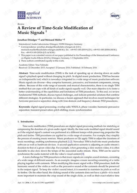
Time-scale modiﬁcation (TSM) procedures are digital signal processing methods for stretching or

compressing the duration of a given audio signal. Ideally, the time-scale modiﬁed signal should sound

as if the original signal’s content was performed at a different tempo while preserving properties like

pitch and timbre. TSM procedures are applied in a wide range of scenarios. For example, they simplify

the process of creating music remixes. Music producers or DJs apply TSM to adjust the durations of

music recordings, enabling synchronous playback [

]. Nowadays TSM is built into music production

software as well as hardware devices. A second application scenario is adjusting an audio stream’s

duration to that of a given video clip. For example, when generating a slow motion video, it is often

desirable to also slow down the tempo of the associated audio stream. Here, TSM can be used to

synchronize the audio material with the video’s visual content [3].

A main challenge for TSM procedures is that music signals are complex sound mixtures, consisting

of a wide range of different sounds. As an example, imagine a music recording consisting of a violin

playing together with castanets. When modifying this music signal with a TSM procedure, both the

harmonic sound of the violin as well as the percussive sound of the castanets should be preserved

in the output signal. To keep the violin’s sound intact, it is essential to maintain its pitch as well as

its timbre. On the other hand, the clicking sound of the castanets does not have a pitch—it is much

more important to maintain the crisp sound of the single clicks, as well as their exact relative time

Appl. Sci. 2016, 6, 57; doi:10.3390/app6020057 www.mdpi.com/journal/applsci

Appl. Sci. 2016, 6, 57 2 of 26

positions, in order to preserve the original rhythm. Retaining these contrasting characteristics usually

requires conceptually different TSM approaches. For example, classical TSM procedures based on

waveform similarity overlap-add (WSOLA) [

] or on the phase vocoder (PV-TSM) [

–

] are capable

of preserving the perceptual quality of harmonic signals to a high degree, but introduce noticeable

artifacts when modifying percussive signals. However, it is possible to substantially reduce artifacts by

combining different TSM approaches. For example, in [

], a given audio signal is ﬁrst separated into

a harmonic and a percussive component. Afterwards, each component is processed with a different

TSM procedure that preserves its respective characteristics. The ﬁnal output signal is then obtained by

superimposing the two intermediate output signals.

Our goals in this article are two-fold. First, we aim to foster an understanding of fundamental

challenges and algorithmic approaches in the ﬁeld of TSM by reviewing well-known TSM methods

and discussing their respective advantages and drawbacks in detail. Second, having identiﬁed the

core issues of these classical procedures, we show—through an example—how to improve on them

by combining different algorithmic ideas. We begin the article by introducing a fundamental TSM

strategy as used in many TSM procedures (Section 2) and discussing a simple TSM approach based

on overlap-add (Section 3). Afterwards, we review two conceptually different TSM methods: the

time-domain WSOLA (Section 4) as well as the frequency-domain PV-TSM (Section 5). We then review

the state-of-the-art TSM procedure from [

] that improves on the quality of both WSOLA as well as

PV-TSM by incorporating harmonic-percussive separation (Section 6). Finally, we point out different

application scenarios for TSM (such as music synchronization and pitch-shifting), as well as various

freely available TSM implementations (Section 7).

2. Fundamentals of Time-Scale Modiﬁcation (TSM)

As mentioned above, a key requirement for time-scale modiﬁcation procedures is that they change

the time-scale of a given audio signal without altering its pitch content. To achieve this goal, many

TSM procedures follow a common fundamental strategy which is sketched in Figure 1. The core idea

is to decompose the input signal into short frames. Having a ﬁxed length, usually in the range of

50 to 100 milliseconds

of audio material, each frame captures the local pitch content of the signal. The

frames are then relocated on the time axis to achieve the actual time-scale modiﬁcation, while, at the

same time, preserving the signal’s pitch.

Signal reconstruction

Original signal Analysis frames Synthesis frames

Time-scale modified

signal

Signal decomposition

Frame relocation &

adaption

Analysis

hopsize

Synthesis

hopsize

Figure 1. Generalized processing pipeline of Time-scale modiﬁcation (TSM) procedures.

More precisely, this process can be described as follows. The input of a TSM procedure is a

discrete-time audio signal

x : Z → R

, equidistantly sampled at a sampling rate of

. Note that

although audio signals typically have a ﬁnite length of

L ∈ N

samples

x(r)

for

r ∈ [

: L −

] :=

{

0, 1,

. . .

L −

}

, for the sake of simplicity, we model them to have an inﬁnite support by deﬁning

x(r) =

0 for

r ∈ Z \ [

: L −

]

. The ﬁrst step of the TSM procedure is to split

into short analysis

Appl. Sci. 2016, 6, 57 3 of 26

frames

m ∈ Z

, each of them having a length of

samples (in the literature, the analysis frames are

sometimes also referred to as grains, see [

]). The analysis frames are spaced by an analysis hopsize

(r) =

(

x(r + mH

), if r ∈ [−N/2 : N/2 − 1],

0, otherwise.

(1)

In a second step, these frames are relocated on the time axis with regard to a speciﬁed synthesis

hopsize

. This relocation accounts for the actual modiﬁcation of the input signal’s time-scale by

a stretching factor

α = H

. Since it is often desirable to have a speciﬁc overlap of the relocated

frames, the synthesis hopsize

is often ﬁxed (common choices are

= N/

2 or

= N/

4) while the

analysis hopsize is given by

= H

/α

. However, simply superimposing the overlapping relocated

frames would lead to undesired artifacts such as phase discontinuities at the frame boundaries and

amplitude ﬂuctuations. Therefore, prior to signal reconstruction, the analysis frames are suitably

adapted to form synthesis frames

. In the ﬁnal step, the synthesis frames are superimposed in order

to reconstruct the actual time-scale modiﬁed output signal y : Z → R of the TSM procedure:

y(r) =

∑

m∈Z

(r − mH

) . (2)

Although this fundamental strategy seems straightforward at a ﬁrst glance, there are many pitfalls

and design choices that may strongly inﬂuence the perceptual quality of the time-scale modiﬁed

output signal. The most obvious question is how to adapt the analysis frames

in order to form the

synthesis frames

. There are many ways to approach this task, leading to conceptually different

TSM procedures. In the following, we discuss several strategies.

3. TSM Based on Overlap-Add (OLA)

3.1. The Procedure

In the general scheme described in the previous section, a straightforward approach would

be to simply deﬁne the synthesis frames

to be equal to the unmodiﬁed analysis frames

This strategy

, however, immediately leads to two problems which are visualized in Figure 2.

First, when

reconstructing the output signal by using Equation

(2)

, the resulting waveform typically

shows discontinuities—perceivable as clicking sounds—at the unmodiﬁed frames’ boundaries.

Second, the

synthesis hopsize

is usually chosen such that the synthesis frames are overlapping.

When superimposing the unmodiﬁed frames—each of them having the same amplitude as the input

signal—this typically leads to an undesired increase of the output signal’s amplitude.

Appl. Sci. 2016, 6, 57 4 of 26

0.1

Time (s)

0 0.05 0.1

0 0.05 0.15 0.18

-1

𝑦

𝑥

Figure 2.

Typical artifacts that occur when choosing the synthesis frames

to be equal to the

analysis frames

. The input signal

is stretched by a factor of

α =

1.8. The output signal

shows

discontinuities (blue oval) and amplitude ﬂuctuations (indicated by blue lines).

A basic TSM procedure should both enforce a smooth transition between frames as well as

compensate for unwanted amplitude ﬂuctuations. The idea of the overlap-add (OLA) TSM procedure is

to apply a window function

to the analysis frames, prior to the reconstruction of the output signal

The task of the window function is to remove the abrupt waveform discontinuities at the the analysis

frames’ boundaries. A typical choice for w is a Hann window function

w(r) =







0.5



1 − cos



2π(r+N/2)

N−1



, if r ∈ [−N/2 : N/2 − 1],

0, otherwise.

(3)

The Hann window has the nice property that

∑

n∈Z



r − n



= 1 , (4)

for all

r ∈ Z

. The principle of the iterative OLA procedure is visualized in Figure 3. For the frame

index

m ∈ Z

, we ﬁrst use Equation

(1)

to compute the

analysis frame

(Figure 3a). Then, we

derive the synthesis frame y

(r) =

w(r) x

(r)

∑

n∈Z

w(r − nH

)

. (5)

The nominator of Equation

(5)

constitutes the actual windowing of the analysis frame by

multiplying it pointwise with the given window function. The denominator normalizes the frame by

the sum of the overlapping window functions, which prevents amplitude ﬂuctuations in the output

signal.

Note that

, when choosing

to be a Hann window and

= N/

2, the denominator always

reduces to one by Equation

(4)

. This is the case in Figure 3b where the synthesis frame’s amplitude

is not scaled before being added to the output signal

. Proceeding to the next analysis frame

m+1

(Figure 3c), this frame is again windowed, overlapped with the preceding synthesis frame, and added

to the output signal (Figure 3d). Note that Figure 3 visualizes the case where the original signal is

compressed (

> H

). Stretching the signal (

< H

) works in exactly the same fashion. In this case,

the analysis frames overlap to a larger degree than the synthesis frames.

Appl. Sci. 2016, 6, 57 5 of 26

𝐻

Kategorie 1: 145 EuroKategorie 1: 145

Euro

Kategorie 1: 145 EuroKategorie 1: 145

Euro

Kategorie 1: 145 EuroKategorie 1: 145

Euro

𝑥

𝑦

𝑥

𝑚

(a)

𝑥

𝑦

(b)

𝑦

𝑚

𝑤

𝑥

𝑦

(c)

𝑦

𝑚

𝑥

𝑚

Time

𝑥

𝑚

𝑥

𝑚+1

𝐻

𝑥

𝑦

(d)

𝑦

𝑚

𝑥

𝑚

𝑥

𝑚+1

𝑦

𝑚+1

Figure 3.

The principle of TSM based on overlap-add (OLA). (

) Input audio signal

with analysis

frame

. The output signal

is constructed iteratively; (

) Application of Hann window function

to the analysis frame

resulting in the synthesis frame

; (

) The next analysis frame

m+1

having a

speciﬁed distance of H

samples from x

; (d) Overlap-add using the speciﬁed synthesis hopsize H

OLA is an example of a time-domain TSM procedure where the modiﬁcations to the analysis

frames are applied purely in the time-domain. In general, time-domain TSM procedures are not only

efﬁcient but also preserve the timbre of the input signal to a high degree. On the downside, output

signals produced by OLA often suffer from other artifacts, as we explain next.

3.2. Artifacts

The OLA procedure is in general not capable of preserving local periodic structures that are

present in the input signal. This is visualized in Figure 4 where a periodic input signal

is stretched by

a factor of

α =

1.8 using OLA. When relocating the analysis frames, the periodic structures of

may not

align any longer in the superimposed synthesis frames. In the resulting output signal

, the periodic

patterns are distorted. These distortions are also known as phase jump artifacts.

Since local

periodicities

in the waveforms of audio signals correspond to harmonic sounds, OLA is not suited to modify signals

that contain harmonic components. When applied to harmonic signals, the output signals of OLA

have a characteristic warbling sound, which is a kind of periodic frequency modulation [

]. Since most

music signals contain at least some harmonic sources (as for example singing voice, piano, violins, or

guitars), OLA is usually not suited to modify music.

剩余25页未读，继续阅读

Michaelliu_dev

粉丝: 490
资源: 9

会员权益专享

A Review of Time-Scale Modification of Music Signals

评论0

会员权益专享

最新资源

A Review of Time-Scale Modification of Music Signals

评论0

Trajectory modification considering dynamic constraints of autonomous robots.pdf

with -lt: sort by, and show, ctime (time of last modification of file status information); with -l: show ctime and sort by name; otherwise: sort by ctime, newest first是什么意思

how to check the latest file modification time under one directory in linux

桌面上有目录A和B，用C++中filesystem对于目录A、B内部的所有同名文件或子目录进行最后修改时间判断，最后修改时间一致的直接略过；

微软内部资料-SQL性能优化3

epoch-dependent dropout

SAE J2284-4-201606

创建改价表记录流水(change_price_logs),字段包括修改人,修改单号,改价金额,修改时间,是否回传OA审批,备注。

Expert PHP and MySQL(Apress,2013)

文件名为时间python读取离当前时间最近的文件

struct stat

这句话是否有语病1. In the paragraph 5 of Introduction, the expression of “Owing to the …… to be similar” is not clear, please make further modification about the high randomness and explain how it affects the performance of loop heat pipes.

Please provide the code of Materials Studio to realize the carboxyl group modification of graphene surface with perl script

Please provide the code of materials studio software to realize the carboxyl group modification of graphene surface with perl script

linux下c语言编程stat

touch -amc 应该怎么记住其分别对应的功能

linux find type

VariFocal Loss

会员权益专享

最新资源