实验模态分析经典资料（AllemangRJ）_实验模态分析

模态分析

需积分: 17 132 浏览量更新于2023-03-16 评论收藏 4.86MB PDF 举报

身份认证购VIP最低享 7 折!

领优惠券(最高得80元）

资源详情

资源评论

资源推荐

CHAPTER 21

EXPERIMENTAL MODAL

ANALYSIS

Randall J. Allemang

David L. Brown

INTRODUCTION

Experimental modal analysis is the process of determining the modal parameters

(natural frequencies, damping factors, modal vectors, and modal scaling) of a linear,

time-invariant system. The modal parameters are often determined by analytical

means, such as finite element analysis. One common reason for experimental modal

analysis is the verification/correction of the results of the analytical approach. Often,

an analytical model does not exist and the modal parameters determined experi-

mentally serve as the model for future evaluations such as structural modifications.

Predominately, experimental modal analysis is used to explain a dynamics problem

(vibration or acoustic) whose solution is not obvious from intuition, analytical mod-

els, or previous experience.

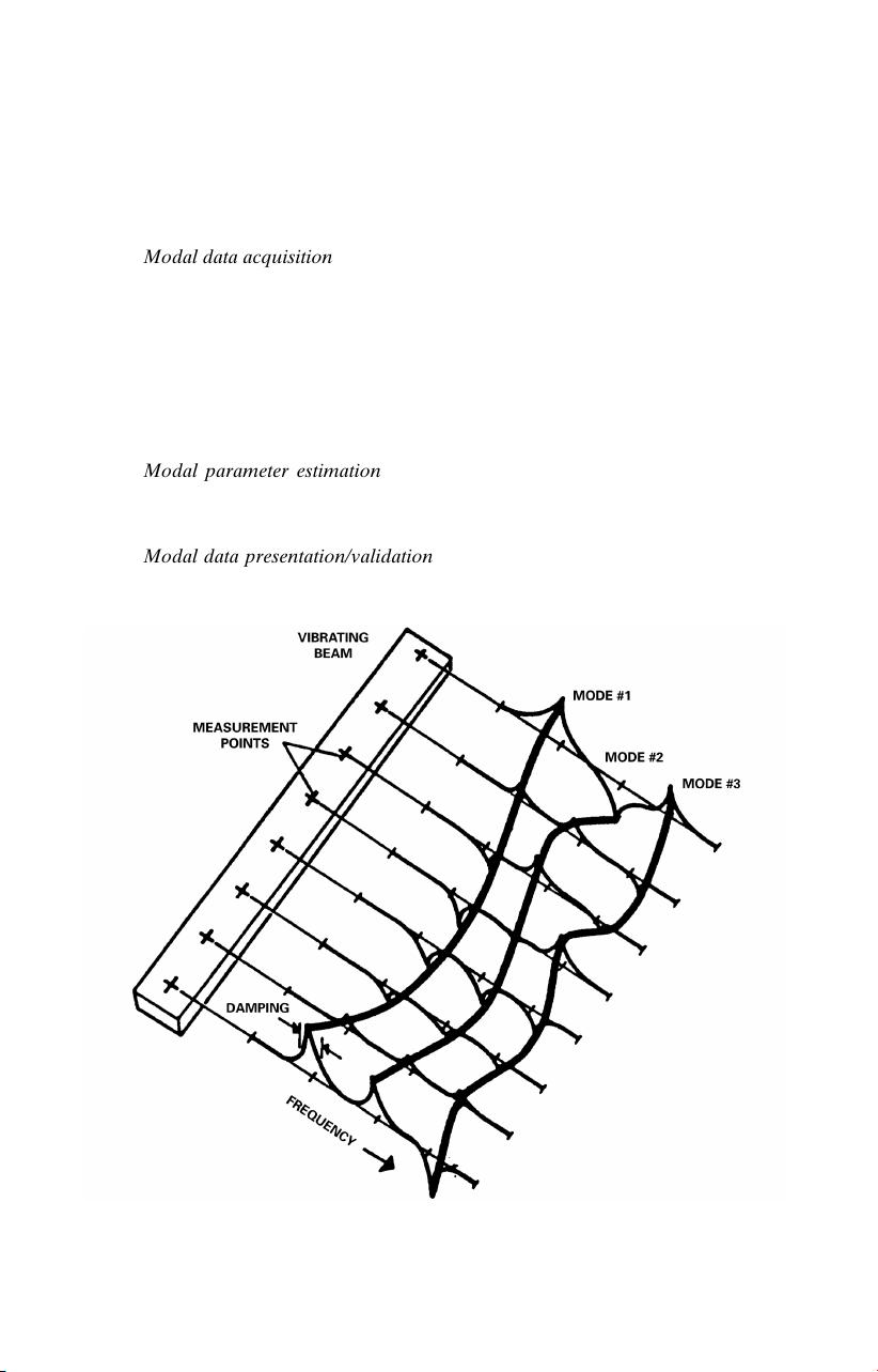
The process of determining modal parameters from experimental data involves

several phases. The success of the experimental modal analysis process depends

upon having very specific goals for the test situation. Every phase of the process is

affected by the goals which are established, particularly with respect to the errors

associated with that phase. One possible delineation of these phases is as follows:

Modal analysis theory refers to that portion of classical vibrations that

explains, theoretically, the existence of natural frequencies, damping factors,

mode shapes, and modal scaling for linear systems. This theory includes both

lumped-parameter, or discrete, models as well as continuous models that rep-

resent the distribution of mass, damping, and stiffness. Since most current

modal parameter estimation methods are based upon frequency response

functions (FRFs) or impulse response functions (IRFs), modal analysis theory

also includes the theoretical definition of these functions with respect to mass,

damping, and stiffness as well. Modal analysis theory also includes the con-

cepts of real normal modes as well as complex modes of vibration as possible

solutions for the modal parameters.

1–3

Experimental modal analysis methods involve the theoretical relationship

between measured quantities and the classic vibration theory often repre-

21.1

Downloaded from Digital Engineering Library @ McGraw-Hill (www.accessengineeringlibrary.com)

Any use is subject to the Terms of Use as given at the website.

Source: HARRIS’ SHOCK AND VIBRATION HANDBOOK

be the numerical tabulation of the frequency, damping, and modal vectors,

along with the associated geometry of the measured degrees of freedom

(DOF). More often, modal data presentation involves the plotting and anima-

tion of such information.

Figure 21.1 is a representation of all phases of the process. In this example, a con-

tinuous beam is being evaluated for the first few modes of vibration. Modal analysis

theory explains that this is a linear system and that the modal vectors of this system

should be real normal modes.The experimental modal analysis method that has been

used is based upon the FRF relationships to the matrix differential equations of

motion. At each measured DOF, the imaginary part of the FRF for that measured

response DOF and a common input DOF is superimposed perpendicular to the beam.

Naturally, the modal data acquisition in this example involves the estimation of FRFs

for each DOF shown.The FRFs are complex-valued functions, and only the imaginary

portion of each function is shown. One method of modal parameter estimation sug-

gests that for systems with light damping and widely spaced modes, the imaginary part

of the FRF, at the damped natural frequency, may be used as an estimate of the modal

coefficient for that response DOF.The damped natural frequency can be identified as

the frequency of the positive and negative peaks in the imaginary part of the FRFs.

The damping can be estimated from the sharpness of the peaks. In this abbreviated

way, the modal parameters have been estimated. Modal data presentation for this case

is shown as the lines connecting the peaks. While animation is possible, a reasonable

interpretation of the modal vector can be gained in this case from plotting alone.

MEASUREMENT DEGREES OF FREEDOM

The development of any theoretical concept in the area of vibrations, including modal

analysis, depends upon an understanding of the concept of the number of degrees of

freedom (n) of a system. This concept is extremely important to the area of modal

analysis, since the number of modes of vibration of a mechanical system is equal to

the number of DOF. From a practical point of view, the relationship between this

theoretical definition of the number of DOF and the number of measurement DOF

) is often confusing. For this reason, the concept of degree of freedom is re-

viewed as a preliminary to the following experimental modal analysis material.

To begin with, the basic definition that is normally associated with the concept of

the number of DOF involves the following statement: The number of degrees of free-

dom for a mechanical system is equal to the number of independent coordinates (or

minimum number of coordinates) that is required to locate and orient each mass in the

mechanical system at any instant in time. As this definition is applied to a point mass,

three DOF are required, since the location of the point mass involves knowing the x,

y, and z translations of the center of gravity of the point mass. As this definition is

applied to a rigid-body mass, six DOF are required, since θ

, θ

, and θ

rotations are

required in addition to the x, y, and z translations in order to define both the orien-

tation and the location of the rigid-body mass at any instant in time. As this defini-

tion is extended to any general deformable body, the number of DOF is essentially

infinite. While this is theoretically true, it is quite common, particularly with respect

to finite element methods, to view the general deformable body in terms of a large

number of physical points of interest, with six DOF for each of the physical points.

In this way, the infinite number of DOF can be reduced to a large but finite number.

When measurement limitations are imposed upon this theoretical concept of the

number of DOF of a mechanical system, the difference between the theoretical

number of DOF (n) and the number of measurement DOF (N

) begins to evolve.

EXPERIMENTAL MODAL ANALYSIS 21.3

Downloaded from Digital Engineering Library @ McGraw-Hill (www.accessengineeringlibrary.com)

Any use is subject to the Terms of Use as given at the website.

EXPERIMENTAL MODAL ANALYSIS

Initially, for a general deformable body, the number of DOF (n) can be considered

to be infinite or equal to some large finite number if a limited set of physical points

of interest is considered, as discussed in the previous paragraph. The first measure-

ment limitation that needs to be considered is that there is normally a limited fre-

quency range that is of interest to the analysis. As this limitation is considered, the

number of DOF of this system that are of interest is now reduced from infinity to a

reasonable finite number.The next measurement limitation that needs to be consid-

ered involves the physical limitation of the measurement system in terms of ampli-

tude. A common limitation of transducers, signal conditioning, and data acquisition

systems results in a dynamic range of 80 to 100 dB (10

to 10

) in the measurement.

This means that the number of DOF is reduced further due to the dynamic range

limitations of the measurement instrumentation. Finally, since few rotational trans-

ducers exist at this time, the normal measurements that are made involve only trans-

lational quantities (displacement, velocity, acceleration, force) and thus do not

include rotational effects, or rotational degrees of freedom (RDOF). In summary,

even for the general deformable body, the theoretical number of DOF that are of

interest is limited to a very reasonable finite value (n = 1 − 50).Therefore, this num-

ber of DOF (n) is the number of modes of vibration that are of interest.

Finally, then, the number of measurement degrees of freedom (N

) can be de-

fined as the number of physical locations at which measurements are made multiplied

by the number of measurements made at each physical location. Since the physical

locations are chosen somewhat arbitrarily, and certainly without exact knowledge of

the modes of vibration that are of interest,there is no specific relationship between the

number of DOF (n) and the number of measurement DOF (N

). In general, in

order to define n modes of vibration of a mechanical system, N

or N

must be equal to

or larger than n. Note also that even though N

or N

is larger than n, this is not a guar-

antee that n modes of vibration can be found from the measurement DOF. The mea-

surement DOF must include physical locations that allow a unique determination of

the n modes of vibration. For example, if none of the measurement DOF are located

on a portion of the mechanical system that is active in one of the n modes of vibration,

portions of the modal parameters for this mode of vibration cannot be found.

In the development of material in the following text, the assumption is made that

a set of measurement DOF exists and allows for n modes of vibration to be deter-

mined. In reality, either N

or N

is always chosen to be much larger than n, since a

prior knowledge of the modes of vibration is not available. If the set of N

or N

mea-

surement degrees of freedom is large enough and if the measurement DOF are dis-

tributed uniformly over the general deformable body, the n modes of vibration are

normally found.

Throughout this experimental modal analysis reference, the frequency response

function H

notation is used to describe the measurement of the response at mea-

surement DOF p resulting from an input applied at measurement DOF q. The sin-

gle subscript p or q refers to a single sensor aligned in a specific direction (X, Y, or

Z) at a physical location on or within the structure.

BASIC ASSUMPTIONS

There are four basic assumptions concerning any structure that are made in order to

perform an experimental modal analysis.

The first basic assumption is that the structure is linear; that is, the response of the

structure to any combination of forces, simultaneously applied, is the sum of the indi-

vidual responses to each of the forces acting alone. For a wide variety of structures,

21.4 CHAPTER TWENTY-ONE

Downloaded from Digital Engineering Library @ McGraw-Hill (www.accessengineeringlibrary.com)

Any use is subject to the Terms of Use as given at the website.

EXPERIMENTAL MODAL ANALYSIS

this is a very good assumption. When a structure is linear, its behavior can be char-

acterized by a controlled excitation experiment in which the forces applied to the

structure have a form convenient for measurement and parameter estimation rather

than being similar to the forces that are actually applied to the structure in its nor-

mal environment. For many important kinds of structures, however, the assumption

of linearity is not valid.Where experimental modal analysis is applied in these cases,

it is hoped that the linear model that is identified provides a reasonable approxima-

tion of the structure’s behavior.

The second basic assumption is that the structure is time invariant; that is, the

parameters that are to be determined are constants. In general, a system which is

not time invariant has components whose mass, stiffness, or damping depends on

factors that are not measured or are not included in the model. For example, some

components may be temperature dependent. In this case, since temperature effects

are not measured, the temperature of the component is an unknown time-varying

signal. Hence, the component has time-varying characteristics. Therefore, the modal

parameters determined by any measurement and estimation process for this case

depend on the time (and the associated temperature dependence) when the mea-

surements are made. If the structure that is tested changes with time, then mea-

surements made at the end of the test period determine a different set of modal

parameters than measurements made at the beginning of the test period. Thus, the

measurements made at the two different times are inconsistent, violating the assump-

tion of time invariance.

The third basic assumption is that the structure obeys Maxwell’s reciprocity; that is,

a force applied at degree of freedom p causes a response at DOF q that is the same

as the response at DOF p caused by the same force applied at DOF q. With respect

to frequency response function measurements, the FRF between points p and q

determined by exciting at p and measuring the response at q is the same FRF found

by exciting at q and measuring the response at p (H

= H

The fourth basic assumption is that the structure is observable; that is, the input/

output measurements that are made contain enough information to generate an ade-

quate behavioral model of the structure. Structures and machines which have loose

components, or, more generally, which have DOF of motion that are not measured,

are not completely observable. For example, consider the motion of a partially filled

tank of liquid when complicated sloshing of the fluid occurs. Sometimes enough data

can be collected so that the system is observable under the form chosen for the

model, while at other times an impractical amount of data is required. This assump-

tion is particularly relevant to the fact that the data normally describes an incom-

plete model of the structure.This occurs in at least two different ways. First, the data

is normally limited to a minimum and maximum frequency as well as a limited fre-

quency resolution.Second, no information is available relative to local rotations due

to a lack of transducers available in this area.

MODAL ANALYSIS THEORY

While modal analysis theory has not changed over the last century, the application of

the theory to experimentally measured data has changed significantly. The advances

of recent years, with respect to measurement and analysis capabilities, have caused a

reevaluation of the aspects of the theory that relate to the practical world of testing.

With this in mind, the aspect of transform relationships has taken on renewed impor-

tance, since digital forms of the integral transforms are in constant use. The theory

EXPERIMENTAL MODAL ANALYSIS 21.5

Downloaded from Digital Engineering Library @ McGraw-Hill (www.accessengineeringlibrary.com)

Any use is subject to the Terms of Use as given at the website.

EXPERIMENTAL MODAL ANALYSIS

剩余53页未读，继续阅读

木兵

粉丝: 0
资源: 1

会员权益专享

实验模态分析经典资料（Allemang RJ）

评论0

会员权益专享

最新资源

实验模态分析 经典资料（Allemang RJ）

评论0

模态分析与实验

实验模态分析及其应用

计算模态分析，实验模态分析

实验模态分析及其应用 pdf

ansys 静态分析 结果作为 模态分析输入

labview做模态分析

ansys陀螺模态分析

ansys模态分析25例

机械振动与模态分析基础许本文pdf

模态分析法matlab

基于matlab的振动模态分析

振动模态分析 pdf

国内外模态分析与模态参数识别的研究现状

ansys 模态分析为0

桥梁模态分析 matlab

workbench模态分析详细教程

dmd模态分析机械震荡

matlab 运行模态分析

ansys模态分析中模态截断是怎样实现的

php入门留言板 php+access PHP语言基础

会员权益专享

最新资源

实验模态分析经典资料（Allemang RJ）

ansys 静态分析结果作为模态分析输入