没有合适的资源?快使用搜索试试~ 我知道了~
首页基于opencv3三维重建教程-英文版
基于opencv3三维重建教程-英文版
需积分: 12 187 浏览量
更新于2023-03-16
评论 2
收藏 1.23MB PDF 举报
opencv3中关于三维重建的经典教程。Packt.OpenCV.3.Computer.Vision.Application.Programming.Cookbook.3rd.Edition.2017.对其单独截取部分
资源详情
资源评论
资源推荐

Chapter 11. Reconstructing 3D
Scenes
In this chapter, we will cover the following recipes:
Calibrating a camera
Recovering camera pose
Reconstructing a 3D scene from calibrated cameras
Computing depth from stereo image
Introduction
We learned in the previous chapter how a camera captures a 3D scene
by projecting light rays on a 2D sensor plane. The image produced is an
accurate representation of what the scene looks like from a particular
point of view, at the instant the image was captured. However, by its
nature, the process of image formation eliminates all information
concerning the depth of the represented scene elements. This chapter
will teach how, under specific conditions, the 3D structure of the scene
and the 3D pose of the cameras that captured it, can be recovered. We
will see how a good understanding of projective geometry concepts
allows us to devise methods that enable 3D reconstruction. We will
therefore revisit the principle of image formation introduced in the
previous chapter; in particular, we will now take into consideration that
our image is composed of pixels.
Digital image formation
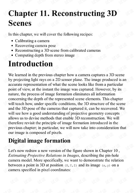
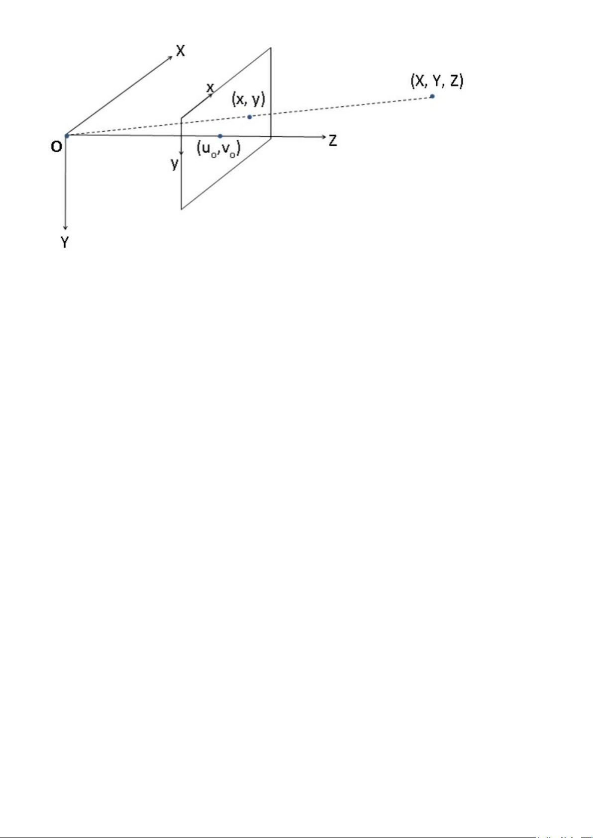
Let's now redraw a new version of the figure shown in Chapter 10 ,
Estimating Projective Relations in Images, describing the pin-hole
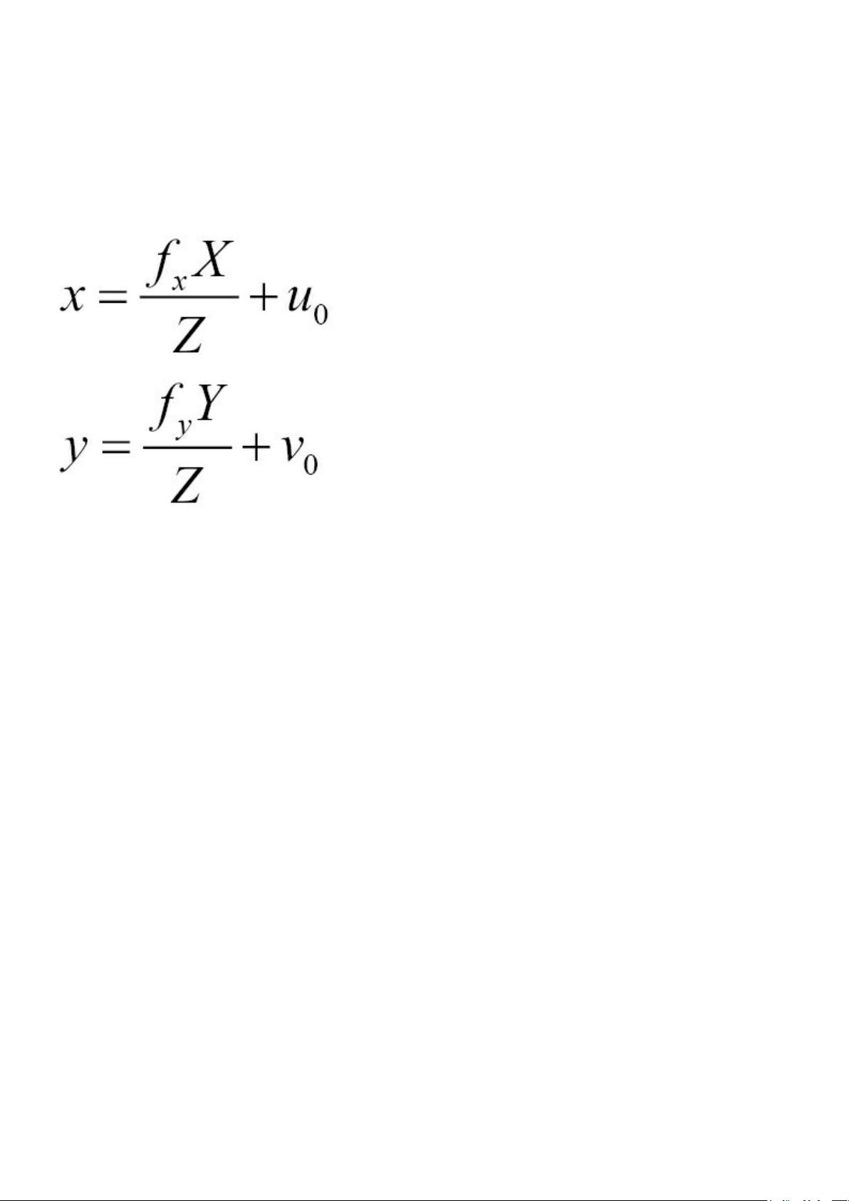
camera model. More specifically, we want to demonstrate the relation
between a point in 3D at position (X,Y,Z) and its image (x,y) on a
camera specified in pixel coordinates:

Notice the changes that have been made to the original figure. First, we
added a reference frame that we positioned at the center of the
projection. Second, we have the Y-axis pointing downward to get a
coordinate system compatible with the usual convention that places the
image origin in the upper-left corner of the image. Finally, we also
identified a special point on the image plane: considering the line coming
from the focal point that is orthogonal to the image plane, the point
(u0,v0) is the pixel position at which this line pierces the image plane.
This point is called the principal point. It could be logical to assume
that this principal point is at the center of the image plane, but in
practice, this one might be off by a few pixels, depending on the
precision with which the camera has been manufactured.
In the previous chapter, we learned that the essential parameters of a
camera in the pin-hole model are its focal length and the size of the
image plane (which defines the field of view of the camera). In addition,
since we are dealing with digital images, the number of pixels on the
image plane (its resolution) is another important characteristic of a
camera. We also learned previously that a 3D point (X,Y,Z) will be
projected onto the image plane at (fX/Z,fY/Z).
Now, if we want to translate this coordinate into pixels, we need to
divide the 2D image position by the pixel width (px) and height (py),

respectively. We notice that by dividing the focal length given in world
units (generally given in millimeters) by px, we obtain the focal length
expressed in (horizontal) pixels. Let's define this term, then, as fx.
Similarly, fy =f/py is defined as the focal length expressed in vertical
pixel units. The complete projective equation is therefore as follows:
Recall that (u0,v0) is the principal point that is added to the result in
order to move the origin to the upper-left corner of the image. Note also
that the physical size of a pixel can be obtained by dividing the size of
the image sensor (generally in millimeters) by the number of pixels
(horizontally or vertically). In modern sensors, pixels are generally
square, that is, they have the same horizontal and vertical size.
The preceding equations can be rewritten in matrix form as we did in
Chapter 10 , Estimating Projective Relations in Images. Here is the
complete projective equation in its most general form:


Calibrating a camera
Camera calibration is the process by which the different camera
parameters (that is, the ones appearing in the projective equation) are
obtained. One can obviously use the specifications provided by the
camera manufacturer, but for some tasks, such as 3D reconstruction,
these specifications are not accurate enough. By undertaking an
appropriate camera calibration step, accurate calibration information
can be obtained.
An active camera calibration procedure will proceed by showing known
patterns to the camera and analyzing the obtained images. An
optimization process will then determine the optimal parameter values
that explain the observations. This is a complex process that has been
made easy by the availability of OpenCV calibration functions.
How to do it...
To calibrate a camera, the idea is to show it a set of scene points for
which their 3D positions are known. Then, you need to observe where
these points project on the image. With the knowledge of a sufficient
number of 3D points and associated 2D image points, the exact camera
parameters can be inferred from the projective equation. Obviously, for
accurate results, we need to observe as many points as possible. One
way to achieve this would be to take one picture of a scene with many
known 3D points, but in practice, this is rarely feasible. A more
convenient way is to take several images of a set of some 3D points
from different viewpoints. This approach is simpler but requires you to
compute the position of each camera view in addition to the
computation of the internal camera parameters, which, fortunately, is
feasible.
OpenCV proposes that you use a chessboard pattern to generate the set
of 3D scene points required for calibration. This pattern creates points at
the corners of each square, and since this pattern is flat, we can freely
assume that the board is located at Z=0, with the X and Y axes well-
剩余40页未读,继续阅读


安全验证
文档复制为VIP权益,开通VIP直接复制

评论0