没有合适的资源?快使用搜索试试~ 我知道了~
首页力导引算法(Force-directed,FDA)详解
资源详情
资源推荐
12
Force-Directed Drawing Algorithms
Stephen G. Kobourov
University of Arizona
12.1 Introduction. . . . . . . . . . . . . . . . . . . . . . . . . . . . . . . . . . . . . . . . . . . . . . . . . 383
12.2 Spring Systems and Electrical Forces . . . . . . . . . . . . . . . . . . . 385
12.3 The Barycentric Method . . . . . . . . . . . . . . . . . . . . . . . . . . . . . . . . . . 386
12.4 Graph Theoretic Distances Approach . . . . . . . . . . . . . . . . . . . 388
12.5 Further Spring Refinements. . . . . . . . . . . . . . . . . . . . . . . . . . . . . . . 389
12.6 Large Graphs . . . . . . . . . . . . . . . . . . . . . . . . . . . . . . . . . . . . . . . . . . . . . . . 391
12.7 Stress Majorization . . . . . . . . . . . . . . . . . . . . . . . . . . . . . . . . . . . . . . . . 396
12.8 Non-Euclidean Approaches . . . . . . . . . . . . . . . . . . . . . . . . . . . . . . . 397
12.9 Lombardi Spring Embedders . . . . . . . . . . . . . . . . . . . . . . . . . . . . . 400
12.10 Dynamic Graph Drawing . . . . . . . . . . . . . . . . . . . . . . . . . . . . . . . . . 401
12.11 Conclusion . . . . . . . . . . . . . . . . . . . . . . . . . . . . . . . . . . . . . . . . . . . . . . . . . . 403
References . . . . . . . . . . . . . . . . . . . . . . . . . . . . . . . . . . . . . . . . . . . . . . . . . . . . . . . . . . 404
12.1 Introduction
Some of the most flexib le algorithms for calculating layouts of simple undirected graphs
belong to a class known as force-directed algorithms. Also known as spring embedders,
such algorithms calculate the l ayout of a graph using only information contained within
the structure of the graph itself, rather than relying on domain-specific knowledge. Graphs
drawn with these algorithms tend t o be aesthetic ally pleasing, exhibit symmetries, and tend
to produce crossing-free layouts for planar graphs. In this chapter we will assume that the
input graphs are simple, connected, undirected graphs and their layouts are straight-line
drawings. Excellent surveys of this topic can be found in Di Battista et al. [DETT99]
Chapter 10 and Brandes [Bra01].
Going back to 1963, the graph drawing algorithm of Tutte [Tut63] is one of the first force-
direct ed graph drawing methods based on barycentric representations. More tr ad iti onally,
the spr in g layout method of Eades [Ead84] and the algorithm of Fruchterman and Rein-
gold [FR91] both rely on spring forces, similar t o those in Hooke’s law. In these methods ,
there are repulsive forces be tween all nodes, but also attractive forces between nodes that
are adjacent.
Alternatively, forces between the nodes can be computed based on thei r graph theoretic
distances, determi ne d by the lengths of shortest paths between them. The algorithm of
Kamada and Kawai [KK89] uses spring forces proportional to the graph theoretic distances.
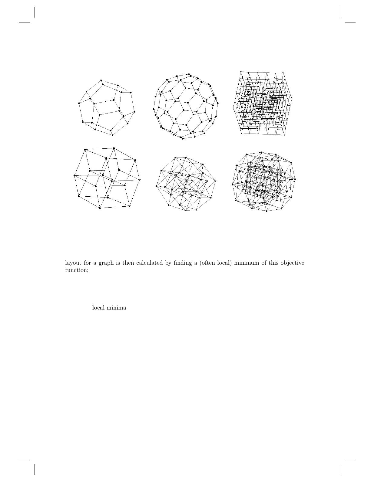
In general, force-directed methods define an objective function which maps each graph
layout into a number in R
+
representing the energy of the layout. This function is defined
in such a way that low energies correspond to layouts in which adjacent nodes are near some
pre-specified distance from each other, and in which non-adjacent no d es ar e well-spaced. A
383
384 CHAPTER 12. FORCE-DIRECTED DRAWING ALGORITHMS
Figure 12.1 Examples of drawings obtained with force-directed algorithms. First row:
small graphs: dodecahedron (20 vertices), C60 bucky ball (60 vertices), 3D cube mesh (216
vertices). Second row: Cubes in 4D, 5D and 6D [GK02].
layout for a graph is then calculated by finding a (often local) minimum of this objective
function; see Figure 12.1.
The utility of the basic f orc e-d ir e ct ed approach is limited to small graphs and results are
poor for graphs with more than a few hundred vertices. There are multiple reasons why
traditional force-directed algorithms do not perfor m well for large graphs. One of the main
obstacles to the scalability of thes e approaches is the fact that the physical model typically
has many local minima. Even with the help of sophisticated mechanisms for avoiding local
minima t he basic force-directed algorithms are not able to consistently produce good layouts
for large graphs. Barycentric methods also do not perform well for large graphs mainly due
to resolution problems: for large graphs the minimum vertex separation tends to be very
small, leading to unreadable drawings.
The late 1990s saw the emergence of several techniques extending the functionality of
force-directed methods to graphs with tens of thousands and even hundreds of thousands of
vertices. One common thread in these approaches is the multi-level layout technique, where
the graph is represented by a series of progressively simpler structures and laid out in reverse
order: from the simplest to the most complex. These structures can be coarser graphs (as in
the approach of Hadany and Harel [HH01], Harel and Koren [HK02], and Walshaw [Wal03],
or vertex filtrations as in the approach of Gajer, Goodrich, and Kobourov [GGK04 ].
The classical force-directed algorithms are restricted to calculating a graph layout in
Euclidean geometry, typically R
2
, R
3
, and, more recently, R
n
for larger values of n. There
are, however, cases where Euclidean geometry may not be the b es t option: Certain graphs
may be known to have a structure which would be best realized in a different geometry,
12.2. SPRING SYSTEMS AND ELECTRICAL FORCES 385
such as on the surface of a sphere or on a torus. In particular, 3D mesh d ata can be
parameterized on the sphere for texture mapping or graphs of genus one can be embedded on
a torus without crossings . Furthermore, it has also been noted that certain non- Euclidean
geometries, s pecifically hyperbolic geometry, have prop er t ies that are particular ly well suited
to the layout and visualization of large classes of graphs [LRP95, Mun97]. With this in mind,
Kobourov and Wampler describe extensions of the force-dir e ct ed algorithms to Riemannian
spaces [KW05].
12.2 Spring S ys tems and Electrical Forces
The 1984 algorithm of Eades [Ead84] targets graphs with up to 30 vertices and uses a
mechanical model to produce “aesthetically pleasing” 2D layouts for plotters and CRT
screens. The algorithm is succinctly summarized as follows:
To embed a graph we replace the vertices by st eel rings and rep lace each edge with
a spring to form a mechanical system. The vertices are placed in some initial
layout and let go so that the spring forces on the rings move the system to a
minimal energy state. Two practical adjustments are made to this idea: firstly,
logarithmic strength spr ings are used; that is, the force exerted by a spring is:
c
1
∗ log(d/c
2
),
where d is the length of the spring, and c
1
and c
2
are constants. Experience
shows that Hookes Law (linear) springs are too strong when the vertices are far
apart; the logarithmic force solves this problem. Note that the springs exert no
force when d = c
2
. Secondly, we make nonadjacent vertices repel each other. An
inverse squa re law force,
c
3
/d
2
,
where c
3
is constant and d is the distance between the vertices, is suitable. The
mechanical system is simulated by the following algorithm.
algorithm SPRI NG(G:graph);
place vertices of G in random locations;
repeat M times
calculate the force on each vertex;
move the vertex c
4
∗ (force on vertex)
draw graph on CRT or plotter.
The values c
1
= 2, c
2
= 1, c
3
= 1, c
4
= 0.1, are appropriate for most graphs.
Almost all grap hs achieve a minimal energy state after the simulation step is
run 100 times, that is, M = 100.
This e xc ell ent descr ip tion encapsulates the essence of spring algorithms and their natural
simplicity, elegance, and conceptual intuitiveness. The goals behind “aesthetically pleasing”
layouts were initially captured by the two criteria: “all the edge lengths ought to be the
same, and the layout should display as much symmetry as pos si bl e.”
The 1991 algorithm of Fruchterman and Reingold added “even vertex distribution” to the
earlier two criteria and treats vertices in the graph as “atomic particles or celestial bodies,
386 CHAPTER 12. FORCE-DIRECTED DRAWING ALGORITHMS
exerting attractive and repulsive force s from one another.” The attractive and repulsive
forces are redefined to
f
a
(d) = d
2
/k, f
r
(d) = −k
2
/d,
in terms of the distance d betwee n two vertices and the optimal distance between vertices
k defined as
k = C
r
area
number of vertices
.
This algorithm is similar to that of Eades in that both algorithms compute attractive
forces between adjacent vertices and repulsive forces between all pairs of vertices. The
algorithm of Fruchterman and Reingold add s the notion of “temperature” which could
be use d as follows: “the temperature could star t at an initial value (say one tenth the
width of the frame) and decay to 0 in an inverse linear fashion.” The temperature controls
the displacement of vertices so that as the layout becomes better, the adjustments become
smaller. The use of temperature here is a special case of a general technique called simu la ted
annealing, whose use in force-directed algorithms is discussed later i n this chapter. The
pseudo-code for the algorithm by Fruchterman and Reingold, shown in Figure 12.2 provides
further insight into the workings of a spring-embedder.
Each iteration the basic algorithm computes O(|E|) attractive forces and O(|V |
2
) repul-
sive forces. To reduce the quadratic complexity of the repulsive forces, Fruchterman and
Reingold suggest using a grid variant of their basic algorithm, where the repulsive forces be-
tween dis tant vertices are ignored. For sparse graphs, and with uniform distribution of the
vertices, this method allows a O(|V |) time approximation to the repulsive forces calculation.
This approach can be thought of as a sp e ci al case of the multi-pole t echnique introduced in
n-body simulations [Gre88] whose use in force-directed algorithms will be furthe r discussed
later in this chapter.
As in the paper by Eades [Ead84] the graphs considered by Fruchterman and Reingold
are small graphs with less than 40 vertic es . The numb e r of iterations of the main loop is
also similar at 50.
12.3 The Barycentric Method
Historically, Tutte’s 1963 barycentric metho d [Tut63] is the first “force-dir ec te d” algorithm
for obtaining a straight-line, crossings free drawing for a given 3-connected planar graph.
Unlike almost all other force-directed methods, Tutte’s guarantees that the resultin g draw-
ing is crossings-free; moreover, all faces of th e drawing are convex.
The idea behind Tutte’s algorithm, shown in Figure 12.3, is that if a face of the planar
graph is fixed in the plane, then suitable positions for the remaining vertices can be found by
solving a system of linear equations, where each vertex posit ion is represented as a convex
combination of the positions of its neighb or s. This algorithm be considered a for ce -di r ec te d
method as summarized in Di Battista et al. [DETT99].
In this model the force due to an edge ( u , v) is propor ti onal to the dis tanc e be tween
vertices u and v and the springs have ideal length of zero; there are no explicit repulsive
forces. Thus the force at a vertex v is describ ed by
F (v) =
X
(u,v)∈E
(p
u
− p
v
),
where p
u
and p
v
are the positions of vertices u and v. As this function has a trivial minimum
with all vertices placed in the same location, the vertex set is partitioned into fixed and free
12.3. THE BARYCENTRIC METHOD 387
area:= W ∗ L; {W and L are the width and length of the frame}
G := (V, E); {the vertices are assi gned random initial positions }
k :=
p
area/|V |;
function f
a
(x) := begin return x
2
/k end;
function f
r
(x) := begin return k
2
/x end;
for i := 1 to iterations do begin
{calculate repulsive forces}
for v in V do begin
{each vertex has two vectors: .pos and .disp
v.disp := 0;
for u in V do
if (u 6= v) then begin
{δ is the d iff er e nc e vector between the pos it ions of the two vertices}
δ := v.pos − u.pos;
v.disp := v.disp + (δ/|δ|) ∗ f
r
(|δ|)
end
end
{calculate attractive forces}
for e in E do begin
{each edges is an ord er e d pair of vertices .vand.u}
δ := e.v.pos − e.u.pos;
e.v.disp := e.v.disp − (δ/|δ|) ∗ f
a
(|δ|);
e.u.disp := e.u.disp + ( δ/|δ|) ∗ f
a
(|δ|)
end
{limit max disp lace ment to temperature t and prevent from displacement
outside frame}
for v in V do begin
v.pos := v.pos + (v.disp/|v.disp|) ∗ min(v.disp, t);
v.pos.x := min(W/2, max(−W/2, v.pos .x )) ;
v.pos.y := min(L/2, max(−L/2, v.pos.y))
end
{reduce the temperature as the layout approaches a bet te r configuration}
t := co o l(t)
end
Figure 12.2 Pseudo-code for the algorithm by Fruchterman and Reingold [FR91].
vertices. Setting the partial derivatives of the force function to zero results in independent
systems of linear equations for the x-coordinate and for the y- coor di nate .
The equations in the for-loop are linear and the number of equations is equal to the
number of the unknowns, which in turn is equal to the number of free vertices. Solving these
equations results in placing each free vertex at the barycenter of its neighbors . The system
of equations can be solved using the Newton-Raphson method. Moreover, the resulting
solution is unique.
One significant drawback of this approach is the resulting drawing often has poor vertex
resolution. In fact, for every n > 1, there exists a graph, such t h at the barycenter method
computes a drawing with exponential area [EG95].
剩余25页未读,继续阅读
Ffanfanm
- 粉丝: 11
- 资源: 3
上传资源 快速赚钱
- 我的内容管理 收起
- 我的资源 快来上传第一个资源
- 我的收益 登录查看自己的收益
- 我的积分 登录查看自己的积分
- 我的C币 登录后查看C币余额
- 我的收藏
- 我的下载
- 下载帮助
会员权益专享
最新资源
- zigbee-cluster-library-specification
- JSBSim Reference Manual
- c++校园超市商品信息管理系统课程设计说明书(含源代码) (2).pdf
- 建筑供配电系统相关课件.pptx
- 企业管理规章制度及管理模式.doc
- vb打开摄像头.doc
- 云计算-可信计算中认证协议改进方案.pdf
- [详细完整版]单片机编程4.ppt
- c语言常用算法.pdf
- c++经典程序代码大全.pdf
- 单片机数字时钟资料.doc
- 11项目管理前沿1.0.pptx
- 基于ssm的“魅力”繁峙宣传网站的设计与实现论文.doc
- 智慧交通综合解决方案.pptx
- 建筑防潮设计-PowerPointPresentati.pptx
- SPC统计过程控制程序.pptx
资源上传下载、课程学习等过程中有任何疑问或建议,欢迎提出宝贵意见哦~我们会及时处理!
点击此处反馈
安全验证
文档复制为VIP权益,开通VIP直接复制
信息提交成功