PetrinetsProperties,analysisandapplications-讲义文档类

需积分: 0 53 浏览量更新于2023-05-29 评论收藏 3.5MB PDF 举报

身份认证购VIP最低享 7 折!

领优惠券(最高得80元）

资源详情

资源评论

资源推荐

Petri Nets: Properties, Analysis and

Appl

kat

ions

TADAO MURATA,

FELLOW,

IEEE

Invited Paper

This is an invited tutorial-review paper on Petri nets-a graphical

and mathematical modeling tool. Petri nets are a promising tool

for describing and studying information processing systems that

are characterized as being concurrent, asynchronous, distributed,

parallel, nondeterministic, and/or stochastic.

The paper starts with

brief review of the history and the appli-

cation areas considered in the literature. It then proceeds with

introductory modeling examples, behavioral and structural prop-

erties, three methods of analysis, subclasses of Petri nets and their

analysis. In particular, one section is devoted to marked graphs-

the concurrent system model most amenable to analysis. In addi-

tion, the paper presents introductory discussions on stochastic nets

with their application

performance modeling, and on high-level

nets with their application

logic programming. Also included

are recent results on reachability criteria. Suggestions are provided

for further reading on many subject areas of Petri nets.

INTRODUCTION

Petri netsareagraphical andmathematical modeling tool

applicable to many systems. They are a promising tool for

describing and studying information processing systems

that are characterized

being concurrent, asynchronous,

distributed, parallel, nondeterministic, and/or stochastic.

As a graphical tool, Petri nets can be used

visual-com-

munication aid similar to flow charts, block diagrams, and

networks. In addition, tokens are used in these nets to sim-

ulate the dynamic and concurrent activities of systems. As

mathematical tool, it

possible to set up state equations,

algebraic equations, and other mathematical models gov-

erning the behavior of systems. Petri nets can be used by

both practitioners and theoreticians. Thus, they provide

powerful medium of communication between them: prac-

titioners can learn from theoreticians how to make their

models more methodical, and theoreticians can learn from

practitioners how to make their models more realistic.

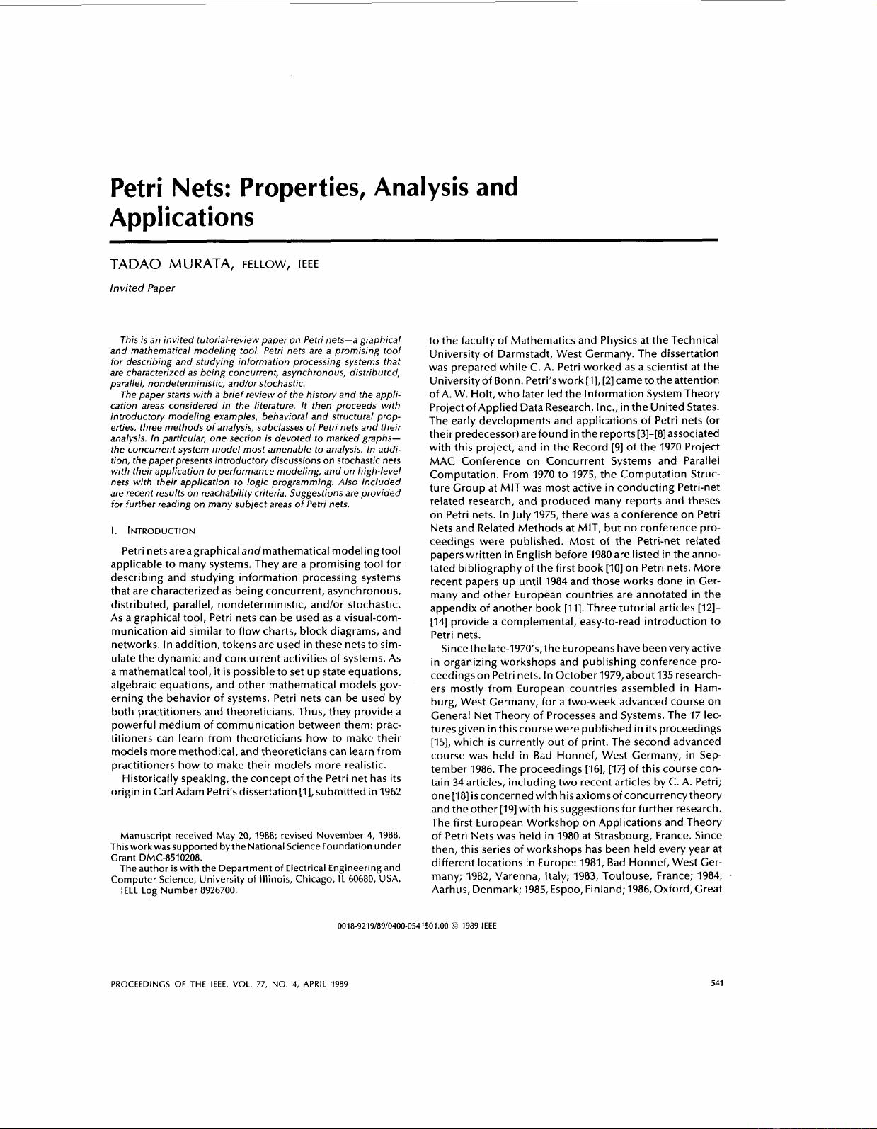
Historically speaking, the concept of the Petri net has its

origin in Carl Adam Petri’s dissertation

[I],

submitted in 1962

Manuscript received May

20,

1988; revised November

1988.

This work was supported by the National Science Foundation under

Grant DMC-8510208.

The author

with the Department

Electrical Engineering and

Computer Science, University

Illinois, Chicago,

60680, USA.

IEEE

Log

Number 8926700.

to the faculty of Mathematics and Physics at the Technical

University of Darmstadt, West Germany. The dissertation

was prepared while

A. Petri worked as a scientist at the

Universityof Bonn. Petri’swork[l], [2]came totheattention

of A. W. Holt, who later led the Information System Theory

Project of Applied Data Research, Inc., in the United States.

The early developments and applications of Petri nets (or

their predecessor)arefound in the reports [3]-[8] associated

with this project, and in the Record [9] of the 1970 Project

MAC Conference on Concurrent Systems and Parallel

Computation. From 1970 to 1975, the Computation Struc-

ture Group at

MIT

was most active in conducting Petri-net

related research, and produced many reports and theses

on Petri nets. In July 1975, there was

conference on Petri

Nets and Related Methods at MIT, but no conference pro-

ceedings were published. Most of the Petri-net related

papers written in English before 1980 are listed in the anno-

tated bibliography of the first book [IO] on Petri nets. More

recent papers up until 1984 and those works done in Ger-

many and other European countries are annotated in the

appendix of another book [Ill. Three tutorial articles [12]-

[I41 provide

complemental, easy-to-read introduction to

Petri nets.

Sincethe late-I970‘s, the Europeans have been veryactive

in organizing workshops and publishing conference pro-

ceedings on Petri nets. In October 1979, about

135

research-

ers mostly from European countries assembled in Ham-

burg, West Germany, for

two-week advanced course on

General Net Theory of Processes and Systems. The 17 lec-

turesgiven in thiscoursewere published in its proceedings

[15], which

currently out of print. The second advanced

course was held in Bad Honnef, West Germany, in Sep-

tember 1986. The proceedings [16],

[I7

of this course con-

tain

articles, including two recent articles by C. A. Petri;

one[l8] isconcerned with hisaxiomsof concurrencytheory

and the other [I91 with his suggestions for further research.

The first European Workshop on Applications and Theory

of Petri Nets was held in 1980 at Strasbourg, France. Since

then, this series of workshops has been held every year at

different locations in Europe: 1981, Bad Honnef, West Ger-

many; 1982, Varenna, Italy; 1983, Toulouse, France; 1984,

Aarhus, Denmark; 1985, Espoo, Finland; 1986, Oxford, Great

0018-9219/89/0400-0541$01.00

1989

IEEE

PROCEEDINGS

THE IEEE, VOL.

77,

NO.

APRIL

1989

541

Britain; 1987, Zaragoza, Spain; 1988, Venice, Italy; and 1989,

Bad Honnef, West Germany (planned). The distribution of

the proceedings of theseworkshops is limited to mostly the

workshop participants. However, selected papers from

these workshops and other articles have been published

by Springer-Verlag as Advances

Petri Nets [20]-[25]. The

1987 volume [24] contains the most comprehensive bibli-

ographyof Petri nets[26] listing2074entries published from

1962 to early1987. The”recent publications” section of Petri

Net Newsletter [27l lists short abstracts of recent publica-

tions three times ayear, and

agood sourceof information

about the most recent Petri net literature.

July 1985, another series of international workshops

was initiated. This series places emphasis on timed and sto-

chastic nets and their applications

performance evalu-

ation. The first internationl workshop on timed Petri nets

was held in Torino, Italy, in July 1985; the second was held

Madison, Wisconsin, in August 1987; the third

to be

held in Kyoto, Japan,

December

1989;

and the fourth

planned in Australia

1991. The proceedings of the first

two workshops [28], [29] are available from the

IEEE

Com-

puter Society Press.

The above

a brief history of Petri nets. Now, we

look

at some application areas considered in the literature. Petri

nets have been proposed for a very wide variety of appli-

cations. This

due

the generality and permissiveness

inherent in Petri nets. They can beapplied informallyto any

area or system that can be described graphically like flow

charts and that needs some means of representing parallel

or concurrent activities. However, careful attention must

be paid

a tradeoff between modeling generalityand anal-

ysis capability. That

is,

the more general the model, the less

amenable

to analysis.

fact, a major weakness of Petri

nets

the complexity problem, i.e., Petri-net-based models

tend to become

too

large for analysis even for a modest-size

system.

applying Petri nets, it

often necessary to add

special modifications

restrictions suited to the particular

application. Two successful application areas are perfor-

mance evaluation [28]-[50] and communication protocols

[51]-[62]. Promising areas of applications include modeling

and analysis of distributed-software systems [63]-[71], dis-

tributed-database systems [72]-[75], concurrent and par-

allel programs [76]-[92], flexible

manufacturing/industrial

control systems [93]-[IOO], discrete-event systems

[loll-

[103], multiprocessor memorysystems [30], [104], [105], data-

flow computing systems [106]-[108], fault-tolerant systems

[log]-[114], programmable logic and VLSl arrays [115]-[120],

asynchronous circuits and structures [121]-[129], compiler

and operating systems [130], [131], office-information sys-

tems [132]-[135], formal languages [136]-[142], and logic pro-

grams [143]-[150]. Other interesting applications consid-

ered in the literature are local-area networks [151]-[153],

legal systems [154], human factors [155], [156], neural net-

works [157], [158], digital filters [159]-[161], and decision

models [162].

The use of computer-aided tools

a necessity for prac-

tical applications of Petri nets. Most Petri-net research

groups have their own software packages and

tools

to assist

the drawing, analysis, and/or simulation of various appli-

cations. A recent article [I631 provides a good overview of

typical Petri-net tools existing as of 1986. Some of these

tools

and their applications are discussed

details in references

[I641 through [170].

The rest of this paper consists of the following topics.

Section

I I

discusses informally the transition enabling and

firing rule with and without capacity constraints. Several

introductory modeling examples are given in Section

Ill

illustrate modeling capabilities and concepts such as con-

flict (choice or decision), concurrency, synchronization, etc.

Section IV describes behavioral or marking-dependent

properties that can be studied using Petri nets. Section V

presents three methods of analysis: the coverability tree,

matrix equations, and reduction techniques. Section

concerned with subclasses of Petri nets and their analysis.

In-depth analysis and synthesis methods are given

Sec-

tion VI

for one of the subclasses known as marked graphs.

Structural or marking-independent properties are

dis-

cussed

Section VIII. Section

presents an introduction

to timed nets, stochastic nets, and high-level nets, together

with their applications. Concluding remarks are given

Section

II.

TRANSITION

ENABLING

AND

FIRING

In this section,wegivetheonly ruleone hastolearn about

Petri-net theory: the rule for transition enabling and firing.

Although this rule appears very simple, its implication in

Petri-net theory

very deep and complex.

A Petrinet

a particular kind of directed graph, together

with an initial state called the initialmarking,

MO.

The under-

lying graph

of a Petri net

a directed, weighted, bipartite

graph consisting of two kinds of nodes, called places and

transitions, where arcs are either from a place toa transition

or from a transition

a place.

graphical representation,

places are drawn as circles, transitions as bars or boxes. Arcs

are labeled with their weights (positive integers), where a

k-weighted arc can be interpreted as the set of

parallel

arcs. Labels for unity weight are usually omitted. A marking

(state)assignstoeach placeanonnegative integer. If amark-

ing assigns to place

a nonnegative integer

we say that

marked with

tokens. Pictorially, we place

black dots

(tokens)

placep. A marking

denoted by

an m-vector,

where

the total number of places. Thepth component

denoted by

M(p),

the number of tokens

placep.

In modeling, using the concept of conditions and events,

places represent conditions, and transitions represent

events. A transition (an event) has acertain number of input

and outputplaces representing the pre-conditions and post-

conditions of the event, respectively. The presence of a

token

a place

interpreted as holding the truth of the

condition associated with the place. In another interpre-

tation,

tokens are put

a place

indicate that

data

items or resources are available. Some typical interpreta-

tions of transitions and their input places and output places

are shown

Table

A formal definition of a Petri net

given

Table 2.

Table

Some Typical Interpretations

Transitions and

Places

Input Places Transition Output Places

Preconditions

Event Postconditions

Input data computation step

Output data

Input signals

Signal processor Output signals

Resources needed

Task or

job

Resources released

Conditions

Clause in logic Conclusion(s)

Buffers

Processor Buffers

542

PROCEEDINGS

THE

IEEE,

VOL.

77,

NO.

APRIL

1989

Table

Formal Definition of a Petri Net

A Petri net is a 5-tuple,

(P,

MO)

where:

{

p,,

p2,

. . .

p,}

is a finite set of places,

{t,,

tZ,

t,}

is a finite set of transitions,

is a set of arcs (flow relation),

--t

(1,

is a weight function,

MO:

(0,

is the initial marking,

0andP

A Petri net structure

(P,

without any specific initial

marking is denoted by

A Petri net with the given initial marking is denoted by

(N,

MO).

The behavior of many systems can be described in terms

of system states and their changes. In order to simulate the

dynamic behavior of a system,

state or marking in a Petri

nets

changed according to the following transition (firing)

rule:

A transition tis said to be enabled if each input place

pof

tismarkedwithatleastw(p,t)tokens,wherew(p,

the weight of the arc from

An enabled transition mayor may not fire(depending

on whether or not the event actually takes place).

A firing of an enabled transition

removes w(p,

tokens from each input place

and adds w(t,

tokens to each output placep of

where w(t,

the

weight of the arc from

A transition without any input place

called a source

transition, and one without any output place

called

sink

transition. Note that a source transition

unconditionally

enabled, and that the firing of a sink transition consumes

tokens, but does not produce any.

A pair of

place

and a transition

called a self-loop

both an input and output place of

A Petri net

said

to be pure if it has no self-loops. A Petri net

said to be

ordinary

all

of its arc weights are

1’s.

€xample

The above transition rule

illustrated in Fig.

using the well-known chemical reaction: 2H2

2H20.

Two tokens in each input place in Fig.

l(a)

show that

two units of

and

are available, and the transition

enabled. After firing

the marking will change to the one

shown in Fig. l(b), where the transition

no longer

enabled.

0‘

H2>

(b)

Fig.

Example

An illustration of a transition (firing) rule:

(a)The marking before firingtheenabled transition

(b)The

marking after firing

where tis disabled.

For the above rule of transition enabling, it

assumed

that each place can accommodate an unlimited number of

tokens. Such

Petri net

referred to

an infinite capacity

net. For modeling many physical systems, it

natural to

consider an upper limit to the number of tokens that each

place can hold. Such

Petri net

referred to as a finite

capacity net. For a finite capacity net

(N,

MO), each place

has an associated capacity

K(p),

the maximum number of

tokens that

can hold at any time. For finite capacity nets,

for a transition

to be enabled, there

an additional con-

dition that the number of tokens in each output place

cannot exceed its capacity

K(p)

after firing

This rule with the capacity constraint

called the strict

transition rule, whereas the rule without the capacity con-

straint

called the (weak) transition rule. Given

finite

capacity net (N,

MO),

possible to apply either the strict

transition rule to the given net

(N,

MO)

or, equivalently, the

weak transition rule to

transformed net

(N’,

M;),

the net

obtained from (N, MO)

bythefollowingcomplementary-place

transformation, where it

assumed that

pure.

Step

Add

complementary place

p’

for each place

where the initial marking of

p’

given by

M@‘)

Step2: Between each transition

and some comple-

mentary places

p’,

draw new arcs

(t,

p’)

(p’,

where w(t,

p’)

w(p,

and w(p’,

w(t,

p),

that the sum of tokens in place

and its com-

plementary place

p’

equals its capacity

K(p)

for

each place

before and after firing the tran-

sition

K(p)

Mo(p).

Example 2: Let

apply the strict transition rule to the

finite-capacity net

(N,

MO)

shown in Fig. 2(a). At the initial

marking

0),

the only enabled transition

tl.

After

firing

t,,

we have

0),

where only

and

are

enabled.

changes to

after firing

t2,

or to M3

after firing

t3.

Continuing this process, it

easy to

drawthe(reachabi1ity)graph

shown in Fig. 2(c), which shows

all

possible markings and all possible firings at each mark-

ing. Now, let

see how the net (N,

MO)

shown in Fig.

2(a)

transformed by the complementary-place transformation

into the net

(N’,

Mi)

shown in Fig. 2(b). The first step

add the two complementary places

and

with their ini-

tial markings

Mi@;)

K(pl)

Mo(pl)

and

Mh(p;)

K(p,)

Mo(p2)

The next step

add new arcs between each transition

and some comple-

mentary places,

as to keep the sum of tokens in each pair

placespiandp;thesameandequal

toK(pi),i

1,2,

before

and after firing

For example, since w(tl,

pl)

we have

w(p;,

tl)

Similarly, w(t,,

p;)

w(pl,

t3)

2 and w(p;,

t3)

w(t3,

p2)

since firing

removes two tokens from

and adds one token in

(we draw the two-weight arc from

top; and the unit-weight arc from

t3).

Likewise, two

additional arcs

(

t,,

pi)

and

(t4,

p;)

are drawn to obtain the

net

(A”,

shown in Fig. 2(b). In

similar manner, as illus-

trated for

(N,

MO),

easy to draw the reachability graph

forthe net(N‘,M& It isalsoeasytoverifythatthetwo reach-

ability graphs are isomorphic, and that the two nets

(N,

MO)

and (N’,

Mi)

are equivalent with respect to the behavior of

The above discussions may be summarized in the fol-

all

possible firing sequences.

lowing theorem.

MURATA:

PETRI

NETS

543

‘3

‘4

Fig.

Example

An illustration of the complementary-

place transformation: (a) A finite-capacity net

(N,

MO).

(b) The

net

(N’,

M’,,)

after the transformation. (c) The reachability

graph for the net

(N,

MO)

shown in

(a).

Theorem

Let

(N,

MO) be

pure finite-capacity net, where

the strict transition rule

to be applied. Let

(N’,

Mi)

be the

net obtained from

(N,

MO)

by the complementary-place

transformation, where the weak transition rule

appli-

cable to

(N’,

Mi).

Then the two nets

(N,

MO)

and (N’,

M;)

are

equivalent in the sense that both have the same set of all

In view of Theorem

every pure finite-capacity net

(N,

MO)

can be transformed into an equivalent net

(N’,

Mi),

where the weak transition rule

applicable, and thus we

only need consider the weak-transition rule. Therefore,

unless otherwise stated, we consider only infinite-capacity

nets with the weak-transition rule in the rest of this paper.

The reason

that

all

properties associated with a finite-

capacity net can be discussed in terms of thosewith an infi-

nite-capacity net using the complementary-place transfor-

mation.

In Theorem

assumed that

Petri net be pure to

avoid confusion since there are many different interpre-

tations of the enabling condition for

self-loop in a finite

capacity net

[171].

But this

not

real restriction, because

a self-loop can be “refined” or transformed into a loop by

introducing

dummy pair of a transition and

place,

illustrated in Fig.

possible firing sequences.

Ill. INTRODUCTORY

MODELING

EXAMPLES

In this section, several

simpleexamplesaregivento

intro-

duce the reader to some basic concepts of Petri nets that

are useful in modeling.

Fig.

Transformation of a self-loop to a loop.

A. Finite-State Machines

Finite-state machines or their state diagrams can be

equivalently represented by a subclass of Petri nets. As an

example of a finite-state machine, consider

vending

machinewhich acceptseither nickelsordimesand sells156

206

candy bars. For simplicity, suppose the vending

machine can hold up to

206.

Then, the state diagram of the

machine can be represented by the Petri net shown in Fig.

where the five states are represented by the five places

Ge~15

candy

log

Deposit

Get

candy

Fig.

A Petri net (a state machine) representing the state

diagram of

vending machine, where coin return transi-

tions are omitted.

labeled with

OF,

56,

IOC,

156, and

206,

and transformations

from one state to another state are shown by transitions

labeled with input conditions, such as “deposit

56.’’

The

initial state

indicated by initially putting a token in the

placep,, with a06 label in this example. Note that each tran-

sition in this net has exactly one incoming arc and exactly

one outgoing arc. The subclass of Petri nets with this prop-

erty

known as state machines. Any finite-state machine

(or its state diagram) can be modeled with a state machine.

The structure of the place

having two (or more) output

transitions t, and t2, as shown in Fig.

referred to

conflict, decision, or choice, depending on applications.

State machines allow the representation of decisions, but

not the synchronization of parallel activities.

Parallel Activities

Parallel activities

concurrency can be easily expressed

in terms of Petri nets. For example, in the Petri net shown

in Fig.

the parallel or concurrent activities represented

544

PROCEEDINGS

THE

IEEE,

VOL.

77,

NO.

APRIL

1989

‘1

‘3

‘2

(a)

Fig.

A Petri-net structure called a conflict, choice, or

decision. It is a structure exhibiting nondeterminism.

by transitions

and

begin at the firing of transition

and

end with the firing of transition

t4.

In general, two transi-

tions are said to be concurrent

they are causally inde-

pendent, i.e., one transition may fire before or after or in

parallel with the other,

in the case of

and

in Fig.

Fig.

Petri net (a marked graph) representing deter-

ministic parallel activities.

It has been pointed out [I721 that concurrency can be

regarded as a binary relation (denoted by

on the set of

eventsA

{el,e2,.

.~jwhichislj~~iexive@,

e,jard

symmetric (e,

e2 implies e,

e,),

but not tran-

sitive (e,

e2 and

e3 do not necessarily imply

e& For example, one may drive

car (event e,) or

walk(event e3)whilesinging(event e2), but onecannot drive

and walk concurrently.

Note that each place in the net shown in Fig.

has exactly

one incoming arc and exactly one outgoing arc. The sub-

class of Petri nets with this property

known as marked

graphs.

Marked graphs allow representation of concur-

rency but not decisions (conflicts).

Two events e, and e2 are in conflict if either e, or e2 can

occur but not both, and they are concurrent if both events

can occur in any order without conflicts.

situation where

conflict and concurrency are mixed

called

confusion.

Two types of confusion are shown in Fig. 7. Fig. 7(a) shows

symmetric confusion, since

two

events

and

are con-

current while each of

and

in conflict with event

t3.

Fig. 7(b) shows an asymmetric confusion, where

con-

current with

but will be in conflict with

fires first.

C. Dataflow Computation

Petri nets call be used to represent not only the flow of

control but also the flow of data. The net shown in Fig.

a Petri-net representation of

dataflow computation.

dataflow computer

one in which instructions are enabled

for execution by the arrival of their operands, and may be

g/&$

‘3

Fig.

Two types of a confusion.

(a)

Symmetric confusion:

and

are concurrent as well as in conflict with

t3.

(b) Asym-

metric confusion:

is concurrent with

but will be in con-

flict with

t3,

fires before t,.

executed concurrently. In the Petri-net representation of

dataflow computation, tokens denote the values of cur-

rent data

well

the availability of data. In the net shown

in Fig.

the instructions represented by transitions

and

a+b

Divide

a-b

is undefined

Subtract

Fig.

A Petri net showing a dataflow computation for

b)/(a

b).

can be executed concurrently and deposit the resulting

data (a

or (a

the respective output places.

D. Communication Protocols

Communication protocols are another area where Petri

nets can be used to represent and specify essential features

of a system. The liveness and safeness properties (see Sec-

tion

of a Petri net are often used as correctness criteria

in communication protocols. The Petri net shown in Fig.

very simple model of

communication protocol

between two processes. Figure

shows the Petri-net rep-

resentation of

nondeterministic wait process where

trl,

tr2,

tout

fires if response

response 2, or no response

received before a specified time

(tout

respectively.

Synchronization Control

multiprocessor or distributed-processing system,

resources and information are shared among several pro-

cessors. This sharing must be controlled or synchronized

to insure the correct operation

the overall system. Petri

nets have been used to model

variety of synchronization

MURATA:

PETRI

NETS

545

剩余39页未读，继续阅读

jiangdmdr

粉丝: 58
资源: 779

会员权益专享

Petri nets Properties, analysis and applications

评论0

会员权益专享

最新资源

Petri nets Properties, analysis and applications

评论0

Petri网标准 ISO/IEC 15909

给出广义随机petri网在可靠性方面应用的英文学术论文

如何开始学习petri网

如何使用petri网建模工具

Petri网的建模与仿真过程

CPN (Color Petri Net） 即有色的Petri网

petri参数优化算法

如何使用petri网建模工具pipe4.3.0

绘制BPIC2017银行数据集相关的Petri网

petri网的监督控制

找一个随机petri网的例子

在petri net中这三者的区别

有色Petri网教程，PPT非常详细，值得一看

Petri Network(PN)分析法的优缺点

在petri net中，系统的state condition situation的区别是什么

着色petri网CPN监视器monitor帮助文件

pet simulink 下载

业务建模与业务流程建模的讲解ppt

网络安全概述(3).ppt

会员权益专享

最新资源

CPN (Color Petri Net）即有色的Petri网