没有合适的资源?快使用搜索试试~ 我知道了~
首页Parameter estimation for text analysis
Parameter estimation for text analysis
5星 · 超过95%的资源 需积分: 9 42 下载量 83 浏览量
更新于2023-03-16
评论
收藏 1.79MB PDF 举报
Parameter estimation for text analysis Gregor Heinrich Parameter estimation for text analysis Gregor Heinrich Parameter estimation for text analysis Gregor Heinrich Parameter estimation for text analysis Gregor Heinrich Parameter estimation for text analysis Gregor Heinrich Parameter estimation for text analysis Gregor Heinrich
资源详情
资源评论
资源推荐
Parameter estimation for text analysis
Gregor Heinrich
Technical Note
vsonix GmbH + University of Leipzig, Germany
gregor@vsonix.com
Abstract. Presents parameter estimation methods common with discrete proba-
bility distributions, which is of particular interest in text modeling. Starting with
maximum likelihood, a posteriori and Bayesian estimation, central concepts like
conjugate distributions and Bayesian networks are reviewed. As an application,
the model of latent Dirichlet allocation (LDA) is explained in detail with a full
derivation of an approximate inference algorithm based on Gibbs sampling, in-
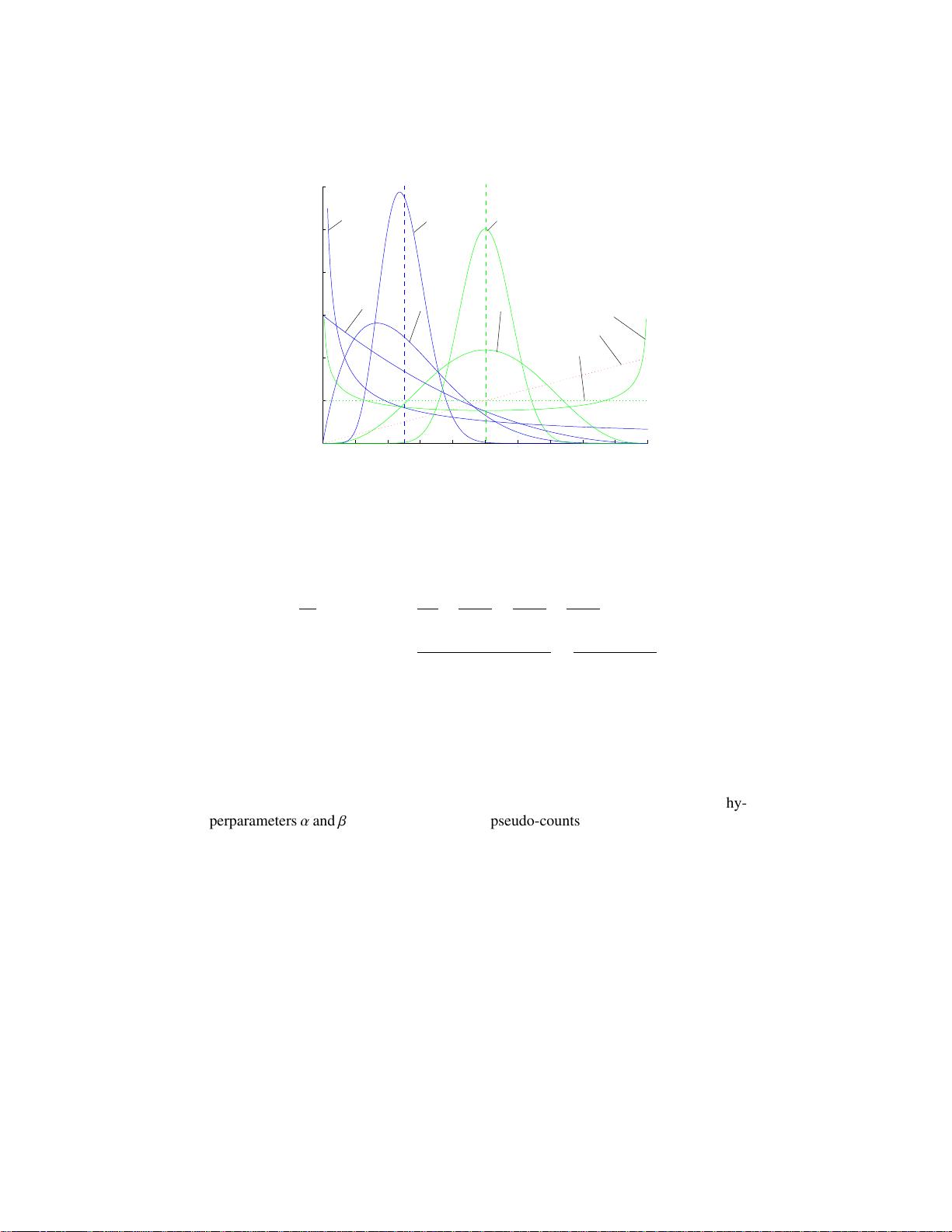
cluding a discussion of Dirichlet hyperparameter estimation.
History: version 1: May 2005, version 2.4: August 2008.
1 Introduction
This technical note is intended to review the foundations of Bayesian parameter esti-
mation in the discrete domain, which is necessary to understand the inner workings of
topic-based text analysis approaches like probabilistic latent semantic analysis (PLSA)
[Hofm99], latent Dirichlet allocation (LDA) [BNJ02] and other mixture models of
count data. Despite their general acceptance in the research community, it appears that
there is no common book or introductory paper that fills this role: Most known texts use
examples from the Gaussian domain, where formulations appear to be rather different.
Other very good introductory work on topic models (e.g., [StGr07]) skips details of
algorithms and other background for clarity of presentation.
We therefore will systematically introduce the basic concepts of parameter estima-
tion with a couple of simple examples on binary data in Section 2. We then will in-
troduce the concept of conjugacy along with a review of the most common probability
distributions needed in the text domain in Section 3. The joint presentation of conjugacy
with associated real-world conjugate pairs directly justifies the choice of distributions
introduced. Section 4 will introduce Bayesian networks as a graphical language to de-
scribe systems via their probabilistic models.
With these basic concepts, we present the idea of latent Dirichlet allocation (LDA)
in Section 5, a flexible model to estimate the properties of text. On the example of
LDA, the usage of Gibbs sampling is shown as a straight-forward means of approximate
inference in Bayesian networks. Two other important aspects of LDA are discussed
afterwards: In Section 6, the influence of LDA hyperparameters is discussed and an
estimation method proposed, and in Section 7, methods are presented to analyse LDA
models for querying and evaluation.
2
2 Parameter estimation approaches
We face two inference problems, (1) to estimate values for a set of distribution param-
eters ϑ that can best explain a set of observations X and (2) to calculate the probability
of new observations ˜x given previous observations, i.e., to find p( ˜x|X). We will refer
to the former problem as the estimation problem and to the latter as the prediction or
regression problem.
The data set X , {x
i
}
|X|
i=1
can be considered a sequence of independent and identi-
cally distributed (i.i.d.) realisations of a random variable (r.v.) X. The parameters ϑ are
dependent on the distributions considered, e.g., for a Gaussian, ϑ = {µ, σ
2
}.
For these data and parameters, a couple of probability functions are ubiquitous in
Bayesian statistics. They are best introduced as parts of Bayes’ rule, which is
1
:
p(ϑ|X) =
p(X|ϑ) · p(ϑ)
p(X)
, (1)
and we define the corresponding terminology:
posterior =
likelihood · prior
evidence
. (2)
In the next paragraphs, we will show different estimation methods that start from simple
maximisation of the likelihood, then show how prior belief on parameters can be incor-
porated by maximising the posterior and finally use Bayes’ rule to infer a complete
posterior distribution.
2.1 Maximum likelihood estimation
Maximum likelihood (ML) estimation tries to find parameters that maximise the likeli-
hood,
L(ϑ|X) , p(X|ϑ) =
\
x∈X
{X = x|ϑ} =
Y
x∈X
p(x|ϑ), (3)
i.e., the probability of the joint event that X generates the data X. Because of the product
in Eq. 3, it is often simpler to use the log likelihood, L , log L. The ML estimation
problem then can be written as:
ˆ
ϑ
ML
= argmax
ϑ
L(ϑ|X) = argmax
ϑ
X
x∈X
log p(x|ϑ). (4)
The common way to obtain the parameter estimates is to solve the system:
∂L(ϑ|X)
∂ϑ
k
!
= 0 ∀ϑ
k
∈ ϑ. (5)
1
Derivation: p(ϑ|X) · p(X) = p(X, ϑ) = p(X|ϑ) · p(ϑ).
Defined as
p(X|θ)
3
The probability of a new observation ˜x given the data X can now be found using the
approximation
2
:
p( ˜x|X) =
Z
ϑ∈Θ
p( ˜x|ϑ) p(ϑ|X) dϑ (6)
≈
Z
ϑ∈Θ
p( ˜x|
ˆ
ϑ
ML
) p(ϑ|X) dϑ = p( ˜x|
ˆ
ϑ
ML
), (7)
that is, the next sample is anticipated to be distributed with the estimated parameters
ˆ
ϑ
ML
.
As an example, consider a set C of N Bernoulli experiments with unknown param-
eter p, e.g., realised by tossing a deformed coin. The Bernoulli density function for the
r.v. C for one experiment is:
p(C=c|p) = p
c
(1 − p)
1−c
, Bern(c|p) (8)
where we define c=1 for heads and c=0 for tails
3
.
Building an ML estimator for the parameter p can be done by expressing the (log)
likelihood as a function of the data:
L = log
N
Y
i=1
p(C=c
i
|p) =
N
X
i=1
log p(C=c
i
|p) (9)
= n
(1)
log p(C=1|p) + n
(0)
log p(C=0|p)
= n
(1)
log p + n
(0)
log(1 − p) (10)
where n
(c)
is the number of times a Bernoulli experiment yielded event c. Differentiating
with respect to (w.r.t.) the parameter p yields:
∂L
∂p
=
n
(1)
p
−
n
(0)
1 − p
!
= 0 ⇔ ˆp
ML
=
n
(1)
n
(1)
+ n
(0)
=
n
(1)
N
, (11)
which is simply the ratio of heads results to the total number of samples. To put some
numbers into the example, we could imagine that our coin is strongly deformed, and
after 20 trials, we have n
(1)
=12 times heads and n
(0)
=8 times tails. This results in an ML
estimation of of ˆp
ML
= 12/20 = 0.6.
2.2 Maximum a posteriori estimation
Maximum a posteriori (MAP) estimation is very similar to ML estimation but allows
to include some a priori belief on the parameters by weighting them with a prior dis-
tribution p(ϑ). The name derives from the objective to maximise the posterior of the
parameters given the data:
ˆ
ϑ
MAP
= argmax
ϑ
p(ϑ|X). (12)
2
The ML estimate
ˆ
ϑ
ML
is considered a constant, and the integral over the parameters given the
data is the total probability that integrates to one.
3
The notation in Eq. 8 is somewhat peculiar because it makes use of the values of c to “filter”
the respective parts in the density function and additionally uses these numbers to represent
disjoint events.
∫p(θ|X) dθ = 1
P就是7式中的θ
4
By using Bayes’ rule (Eq. 1), this can be rewritten to:
ˆ
ϑ
MAP
= argmax
ϑ
p(X|ϑ)p(ϑ)
p(X)
p(X) , f (ϑ)
= argmax
ϑ
p(X|ϑ)p(ϑ) = argmax
ϑ
{L(ϑ|X) + log p(ϑ)}
= argmax
ϑ
n
X
x∈X
log p(x|ϑ) + log p(ϑ)
o
. (13)
Compared to Eq. 4, a prior distribution is added to the likelihood. In practice, the prior
p(ϑ) can be used to encode extra knowledge as well as to prevent overfitting by enforc-
ing preference to simpler models, which is also called Occam’s razor
4
.
With the incorporation of p(ϑ), MAP follows the Bayesian approach to data mod-
elling where the parameters ϑ are thought of as r.v.s. With priors that are parametrised
themselves, i.e., p(ϑ) := p(ϑ|α) with hyperparameters α, the belief in the anticipated
values of ϑ can be expressed within the framework of probability
5
, and a hierarchy of
parameters is created.
MAP parameter estimates can be found by maximising the term L(ϑ|X) + log p(ϑ),
similar to Eq. 5. Analogous to Eq. 7, the probability of a new observation, ˜x, given the
data, X, can be approximated using:
p( ˜x|X) ≈
Z
ϑ∈Θ
p( ˜x|
ˆ
ϑ
MAP
) p(ϑ|X) dϑ = p( ˜x|
ˆ
ϑ
MAP
). (14)
Returning to the simplistic demonstration on ML, we can give an example for the
MAP estimator. Consider the above experiment, but now there are values for p that
we believe to be more likely, e.g., we believe that a coin usually is fair. This can be
expressed as a prior distribution that has a high probability around 0.5. We choose the
beta distribution:
p(p|α, β) =
1
B(α, β)
p
α−1
(1 − p)
β−1
, Beta(p|α, β), (15)
with the beta function B(α, β) =
Γ(α)Γ(β)
Γ(α+β)
. The function Γ(x) is the Gamma function,
which can be understood as a generalisation of the factorial to the domain of real num-
bers via the identity x! = Γ(x + 1). The beta distribution supports the interval [0,1] and
therefore is useful to generate normalised probability values. For a graphical represen-
tation of the beta probability density function (pdf), see Fig. 1. As can be seen, with
different parameters the distribution takes on quite different pdfs.
In our example, we believe in a fair coin and set α = β = 5, which results in a
distribution with a mode (maximum) at 0.5. The optimisation problem now becomes
4
Pluralitas non est ponenda sine necessitate = Plurality should not be posited without necessity.
Occam’s razor is also called the principle of parsimony.
5
Belief is not identical to probability, which is one of the reasons why Bayesian approaches are
disputed by some theorists despite their practical importance.
与θ无关的去掉
奥卡姆剃刀常用于两种假说的取舍上:如果对于同一现象
有两种不同的假说,我们应该采取比较简单的那一种。
自随机变量?
归一化概率
θ<=>P
已知P(θ)的两点分布?
5
0 0.1 0.2 0.3 0.4 0.5 0.6 0.7 0.8 0.9 1
0
1
2
3
4
5
6
Beta(20, 20)
Beta(1, 1)
Beta(2/3, 2/3)
Beta(10, 30)
Beta(2, 6)
Beta(1/3, 1)
Beta(1, 3)
Beta(2, 1)
Beta(4, 4)
p(p)
p
Fig. 1. Density functions of the beta distribution with different symmetric and asym-
metric parametrisations.
(cf. Eq. 11):
∂
∂p
L + log p(p) =
n
(1)
p
−
n
(0)
1 − p
+
α − 1
p
−
β − 1
1 − p
!
= 0 (16)
⇔ ˆp
MAP
=
n
(1)
+ α − 1
n
(1)
+ n
(0)
+ α + β − 2
=
n
(1)
+ 4
n
(1)
+ n
(0)
+ 8
(17)
This result is interesting in two aspects. The first one is the changed behaviour of the
estimate ˆp
MAP
w.r.t. the counts n
(c)
: their influence on the estimate is reduced by the
additive values that “pull” the value towards ˆp
MAP
= 4/8 = 0.5. The higher the values
of the hyperparameters α and β, the more actual observations are necessary to revise the
belief expressed by them. The second interesting aspect is the exclusive appearance of
the sums n
(1)
+ α − 1 and n
(0)
+ β − 1: It is irrelevant whether the counts actually derive
from actual observations or prior belief expressed as hypervariables. This is why the hy-
perparameters α and β are often referred to as pseudo-counts. The higher pseudo-counts
exist, the sharper the beta distribution is concentrated around its maximum. Again, we
observe in 20 trials n
(1)
=12 times heads and n
(0)
=8 times tails. This results in an MAP
estimation of ˆp
MAP
= 16/28 = 0.571, which in comparison to ˆp
ML
= 0.6 shows the
influence of the prior belief of the “fairness” of the coin.
2.3 Bayesian estimation
Bayesian estimation extends the MAP approach by allowing a distribution over the pa-
rameter set ϑ instead of making a direct estimate. Not only encodes this the maximum
(a posteriori) value of the data-generated parameters, but it also incorporates expec-
tation as another parameter estimate as well as variance information as a measure of
剩余30页未读,继续阅读
-柚子皮-
- 粉丝: 1w+
- 资源: 98
上传资源 快速赚钱
- 我的内容管理 收起
- 我的资源 快来上传第一个资源
- 我的收益 登录查看自己的收益
- 我的积分 登录查看自己的积分
- 我的C币 登录后查看C币余额
- 我的收藏
- 我的下载
- 下载帮助
会员权益专享
最新资源
- RTL8188FU-Linux-v5.7.4.2-36687.20200602.tar(20765).gz
- c++校园超市商品信息管理系统课程设计说明书(含源代码) (2).pdf
- 建筑供配电系统相关课件.pptx
- 企业管理规章制度及管理模式.doc
- vb打开摄像头.doc
- 云计算-可信计算中认证协议改进方案.pdf
- [详细完整版]单片机编程4.ppt
- c语言常用算法.pdf
- c++经典程序代码大全.pdf
- 单片机数字时钟资料.doc
- 11项目管理前沿1.0.pptx
- 基于ssm的“魅力”繁峙宣传网站的设计与实现论文.doc
- 智慧交通综合解决方案.pptx
- 建筑防潮设计-PowerPointPresentati.pptx
- SPC统计过程控制程序.pptx
- SPC统计方法基础知识.pptx
资源上传下载、课程学习等过程中有任何疑问或建议,欢迎提出宝贵意见哦~我们会及时处理!
点击此处反馈
安全验证
文档复制为VIP权益,开通VIP直接复制
信息提交成功
评论2