没有合适的资源?快使用搜索试试~ 我知道了~
首页CS294A Lecture notes Sparse autoencoder (稀疏自编码器课程讲义,吴恩达)
CS294A Lecture notes Sparse autoencoder (稀疏自编码器课程讲义,吴恩达)
需积分: 50 39 下载量 108 浏览量
更新于2023-03-16
评论 4
收藏 414KB PDF 举报
CS294A Lecture notes Sparse autoencoder,Andrew Ng,Stanford University
资源详情
资源评论
资源推荐

CS294A Lecture notes
Andrew Ng
Sparse autoencoder
1 Introduction
Supervised learning is one of the most powerful to ols of AI, and has led to
automatic zip code recognition, speech recognition, self-driving cars, and a
continually improving understanding of the human genome. Despite its sig-
nificant successes, supervised learning today is still severely limited. Specifi-
cally, most applications of it still require that we manually specify the input
features x given to the algorithm. Once a good feature representation is
given, a supervised learning algorithm can do well. But in such domains as
computer vision, audio processing, and natural language processing, there’re
now hundreds or perhaps thousands of researchers who’ve sp ent years of their
lives slowly and laboriously hand-engineering vision, audio or text features.
While much of this feature-engineering work is extremely clever, one has to
wonder if we can do better. Certainly this labor-intensive hand-engineering
approach does not scale well to new problems; further, ideally we’d like to
have algorithms that can automatically le arn even be tter feature representa-
tions than the hand-engineered ones.
These notes describe the sparse autoencoder learning algorithm, which
is one approach to automatically learn features from unlabeled data. In some
domains, such as computer vision, this approach is not by itself competitive
with the best hand-engineered features, but the features it can learn do turn
out to be useful for a range of problems (including ones in audio, text, etc).
Further, there’re more sophisticated versions of the sparse auto encoder (not
described in these notes, but that you’ll hear more about later in the class)
that do surprisingly well, and in many cases are competitive with or superior
to even the best hand-engineered representations.
1

These notes are organized as follows. We will first describe feedforward
neural networks and the backpropagation algorithm for supervised learning.
Then, we show how this is used to construct an autoencoder, which is an
unsupervised learning algorithm. Finally, we build on this to derive a sparse
autoencoder. Because these notes are fairly notation-heavy, the last page
also contains a summary of the symbols used.
2 Neural networks
Consider a supervised learning problem where we have access to labeled train-
ing examples (x
(i)
, y
(i)
). Neural networks give a way of defining a complex,
non-linear form of hypotheses h
W,b
(x), with parameters W, b that we can fit
to our data.
To describe neural networks, we will begin by describing the simplest
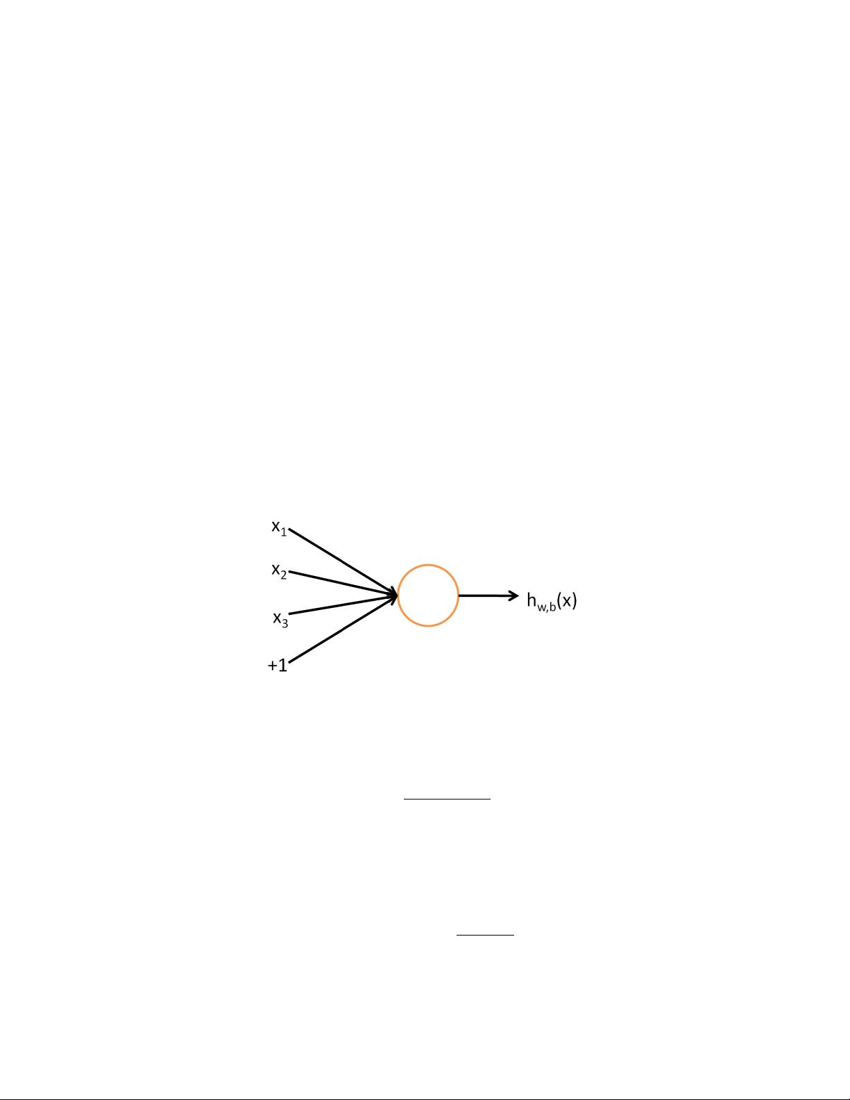
possible neural network, one which comprises a single “neuron.” We will use
the following diagram to denote a single neuron:
This “neuron” is a computational unit that takes as input x
1
, x
2
, x
3
(and
a +1 intercept term), and outputs h
W,b
(x) = f(W
T
x) = f(
P
3
i=1
W
i
x
i
+ b),
where f : R 7→ R is called the activation function. In these notes, we will
choose f(·) to be the sigmoid function:
f(z) =
1
1 + exp(−z)
.
Thus, our single neuron corresponds exactly to the input-output mapping
defined by logistic regression.
Although these notes will use the sigmoid function, it is worth noting that
another common choice for f is the hyperbolic tangent, or tanh, function:
f(z) = tanh(z) =
e
z
− e
−z
e
z
+ e
−z
, (1)
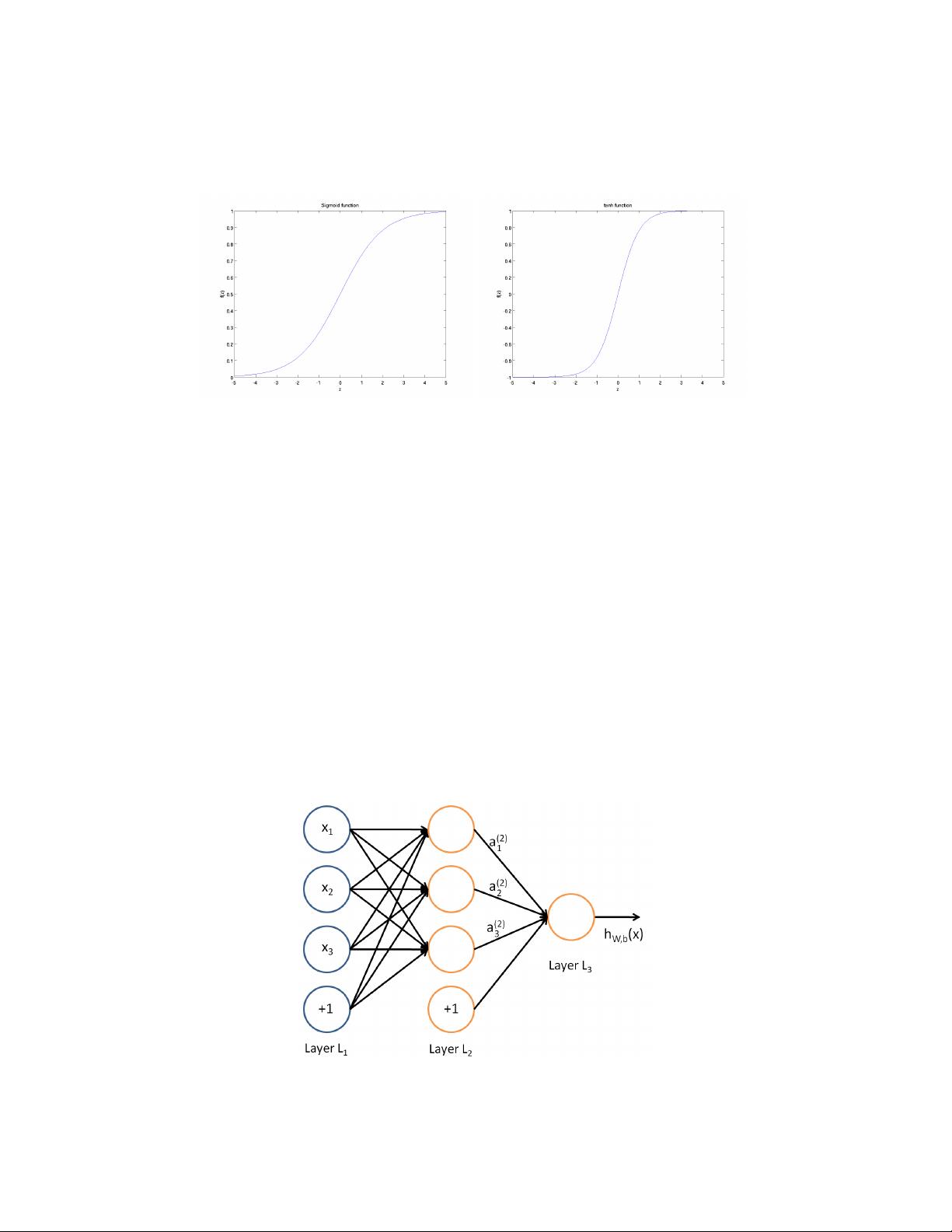
Here are plots of the sigmoid and tanh functions:
2

The tanh(z) function is a rescaled version of the sigmoid, and its output
range is [−1, 1] instead of [0, 1].
Note that unlike CS221 and (parts of) CS229, we are not using the con-
vention here of x
0
= 1. Instead, the intercept term is handled separately by
the parameter b.
Finally, one identity that’ll be useful later: If f(z) = 1/(1 + exp(−z)) is
the sigmoid function, then its derivative is given by f
0
(z) = f(z)(1 − f(z)).
(If f is the tanh function, then its derivative is given by f
0
(z) = 1 − (f(z))
2
.)
You can derive this yourself using the definition of the sigmoid (or tanh)
function.
2.1 Neural network formulatio n
A neural network is put together by hooking together many of our simple
“neurons,” so that the output of a neuron can be the input of another. For
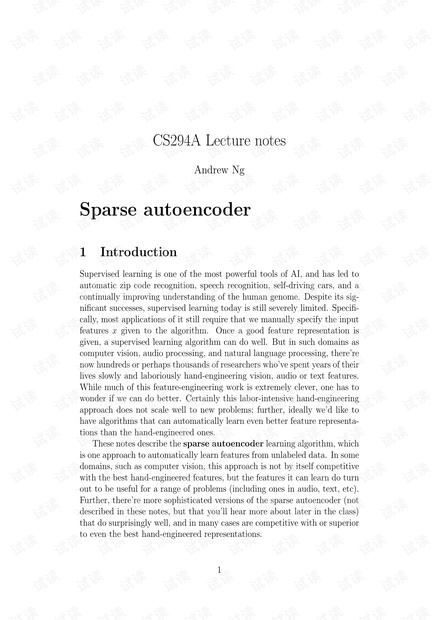
example, here is a small neural network:
3

In this figure, we have used circles to also denote the inputs to the net-
work. The circles labeled “+1” are called bias units, and correspond to the
intercept term. The leftmost layer of the network is called the input layer,
and the rightmost layer the output layer (which, in this example, has only
one node). The middle layer of nodes is called the hidden layer, because
its values are not observed in the training set. We also say that our example
neural network has 3 input units (not counting the bias unit), 3 hidden
units, and 1 output unit.
We will let n
l
denote the number of layers in our network; thus n
l
= 3
in our example. We label layer l as L
l
, so layer L
1
is the input layer, and
layer L
n
l
the output layer. Our neural network has parameters (W, b) =
(W
(1)
, b
(1)
, W
(2)
, b
(2)
), where we write W
(l)
ij
to denote the parameter (or weight)
associated with the connection between unit j in layer l, and unit i in layer
l+1. (Note the order of the indices.) Also, b
(l)
i
is the bias associated with unit
i in layer l+1. Thus, in our example, we have W
(1)
∈ R
3×3
, and W
(2)
∈ R
1×3
.
Note that bias units don’t have inputs or connections going into them, since
they always output the value +1. We also let s
l
denote the number of nodes
in layer l (not counting the bias unit).
We will write a
(l)
i
to denote the activation (meaning output value) of
unit i in layer l. For l = 1, we also use a
(1)
i
= x
i
to denote the i-th input.
Given a fixed setting of the parameters W, b, our neural ne twork defines a
hypothesis h
W,b
(x) that outputs a real number. Specifically, the computation
that this neural network represents is given by:
a
(2)
1
= f(W
(1)
11
x
1
+ W
(1)
12
x
2
+ W
(1)
13
x
3
+ b
(1)
1
) (2)
a
(2)
2
= f(W
(1)
21
x
1
+ W
(1)
22
x
2
+ W
(1)
23
x
3
+ b
(1)
2
) (3)
a
(2)
3
= f(W
(1)
31
x
1
+ W
(1)
32
x
2
+ W
(1)
33
x
3
+ b
(1)
3
) (4)
h
W,b
(x) = a
(3)
1
= f(W
(2)
11
a
(2)
1
+ W
(2)
12
a
(2)
2
+ W
(2)
13
a
(2)
3
+ b
(2)
1
) (5)
In the sequel, we also let z
(l)
i
denote the total weighted sum of inputs to unit
i in layer l, including the bias term (e.g., z
(2)
i
=
P
n
j=1
W
(1)
ij
x
j
+ b
(1)
i
), so that
a
(l)
i
= f(z
(l)
i
).
Note that this easily lends itself to a more compact notation. Specifically,
if we extend the activation function f(·) to apply to vectors in an element-
wise fashion (i.e., f([z
1
, z
2
, z
3
]) = [f(z
1
), f(z
2
), f(z
3
)]), then we can write
4
剩余18页未读,继续阅读
物幻物移
- 粉丝: 0
- 资源: 9
上传资源 快速赚钱
 我的内容管理
收起
 我的资源
快来上传第一个资源
 我的收益 登录查看自己的收益
 我的积分
登录查看自己的积分
 我的C币
登录后查看C币余额
 我的收藏
我的收藏  我的下载
我的下载  下载帮助
下载帮助

会员权益专享
最新资源
- stc12c5a60s2 例程
- Android通过全局变量传递数据
- c++校园超市商品信息管理系统课程设计说明书(含源代码) (2).pdf
- 建筑供配电系统相关课件.pptx
- 企业管理规章制度及管理模式.doc
- vb打开摄像头.doc
- 云计算-可信计算中认证协议改进方案.pdf
- [详细完整版]单片机编程4.ppt
- c语言常用算法.pdf
- c++经典程序代码大全.pdf
- 单片机数字时钟资料.doc
- 11项目管理前沿1.0.pptx
- 基于ssm的“魅力”繁峙宣传网站的设计与实现论文.doc
- 智慧交通综合解决方案.pptx
- 建筑防潮设计-PowerPointPresentati.pptx
- SPC统计过程控制程序.pptx
资源上传下载、课程学习等过程中有任何疑问或建议,欢迎提出宝贵意见哦~我们会及时处理!
点击此处反馈


安全验证
文档复制为VIP权益,开通VIP直接复制
 信息提交成功
评论0