没有合适的资源?快使用搜索试试~ 我知道了~
首页Deep Reinforcement Learning in Large Discrete Action Spaces
Deep Reinforcement Learning in Large Discrete Action Spaces
需积分: 16 8 下载量 130 浏览量
更新于2023-03-16
评论
收藏 1.38MB PDF 举报
Deep Reinforcement Learning in Large Discrete Action Spaces论文
资源详情
资源评论
资源推荐
Deep Reinforcement Learning in Large Discrete Action Spaces
Gabriel Dulac-Arnold*, Richard Evans*, Hado van Hasselt, Peter Sunehag, Timothy Lillicrap, Jonathan Hunt,
Timothy Mann, Theophane Weber, Thomas Degris, Ben Coppin DULACARNOLD@GOOGLE.COM
Google DeepMind
Abstract
Being able to reason in an environment with a
large number of discrete actions is essential to
bringing reinforcement learning to a larger class
of problems. Recommender systems, industrial
plants and language models are only some of the
many real-world tasks involving large numbers
of discrete actions for which current methods are
difficult or even often impossible to apply.
An ability to generalize over the set of actions
as well as sub-linear complexity relative to the
size of the set are both necessary to handle such
tasks. Current approaches are not able to provide
both of these, which motivates the work in this
paper. Our proposed approach leverages prior
information about the actions to embed them in
a continuous space upon which it can general-
ize. Additionally, approximate nearest-neighbor
methods allow for logarithmic-time lookup com-
plexity relative to the number of actions, which is
necessary for time-wise tractable training. This
combined approach allows reinforcement learn-
ing methods to be applied to large-scale learn-
ing problems previously intractable with current
methods. We demonstrate our algorithm’s abili-
ties on a series of tasks having up to one million
actions.
1. Introduction
Advanced AI systems will likely need to reason with a large
number of possible actions at every step. Recommender
systems used in large systems such as YouTube and Ama-
zon must reason about hundreds of millions of items every
second, and control systems for large industrial processes
may have millions of possible actions that can be applied
at every time step. All of these systems are fundamentally
*Equal contribution.
reinforcement learning (Sutton & Barto, 1998) problems,
but current algorithms are difficult or impossible to apply.
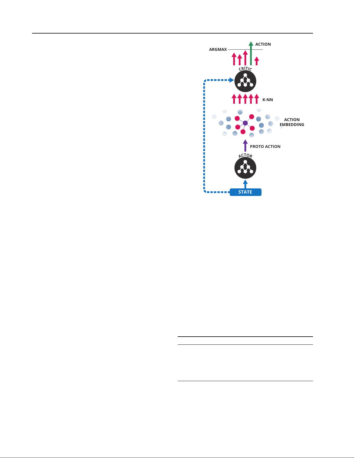
In this paper, we present a new policy architecture which
operates efficiently with a large number of actions. We
achieve this by leveraging prior information about the ac-
tions to embed them in a continuous space upon which the
actor can generalize. This embedding also allows the pol-
icy’s complexity to be decoupled from the cardinality of
our action set. Our policy produces a continuous action
within this space, and then uses an approximate nearest-
neighbor search to find the set of closest discrete actions
in logarithmic time. We can either apply the closest ac-
tion in this set directly to the environment, or fine-tune this
selection by selecting the highest valued action in this set
relative to a cost function. This approach allows for gen-
eralization over the action set in logarithmic time, which is
necessary for making both learning and acting tractable in
time.
We begin by describing our problem space and then detail
our policy architecture, demonstrating how we can train it
using policy gradient methods in an actor-critic framework.
We demonstrate the effectiveness of our policy on various
tasks with up to one million actions, but with the intent that
our approach could scale well beyond millions of actions.
2. Definitions
We consider a Markov Decision Process (MDP) where A is
the set of discrete actions, S is the set of discrete states, P :
S ×A×S → R is the transition probability distribution,
R : S ×A → R is the reward function, and γ ∈ [0, 1] is
a discount factor for future rewards. Each action a ∈ A
corresponds to an n-dimensional vector, such that a ∈ R
n
.
This vector provides information related to the action. In
the same manner, each state s ∈ S is a vector s ∈ R
m
.
The return of an episode in the MDP is the discounted
sum of rewards received by the agent during that episode:
R
t
=
P
T
i=t
γ
i−t
r(s
i
, a
i
). The goal of RL is to learn a
policy π : S → A which maximizes the expected return
over all episodes, E[R
1
]. The state-action value function
Q
π
(s, a) = E[R
1
|s
1
= s, a
1
= a, π] is the expected re-
arXiv:1512.07679v2 [cs.AI] 4 Apr 2016
Deep Reinforcement Learning in Large Discrete Action Spaces
turn starting from a given state s and taking an action a,
following π thereafter. Q
π
can be expressed in a recursive
manner using the Bellman equation:
Q
π
(s, a) = r(s, a) + γ
X
s
0
P (s
0
|s, a)Q
π
(s
0
, π(s
0
)).
In this paper, both Q and π are approximated by
parametrized functions.
3. Problem Description
There are two primary families of policies often used in RL
systems: value-based, and actor-based policies.
For value-based policies, the policy’s decisions are directly
conditioned on the value function. One of the more com-
mon examples is a policy that is greedy relative to the value
function:
π
Q
(s) = arg max
a∈A
Q(s, a). (1)
In the common case that the value function is a parame-
terized function which takes both state and action as input,
|A| evaluations are necessary to choose an action. This
quickly becomes intractable, especially if the parameter-
ized function is costly to evaluate, as is the case with deep
neural networks. This approach does, however, have the
desirable property of being capable of generalizing over
actions when using a smooth function approximator. If a
i
and a
j
are similar, learning about a
i
will also inform us
about a
j
. Not only does this make learning more efficient,
it also allows value-based policies to use the action features
to reason about previously unseen actions. Unfortunately,
execution complexity grows linearly with |A| which ren-
ders this approach intractable when the number of actions
grows significantly.
In a standard actor-critic approach, the policy is explicitly
defined by a parameterized actor function: π
θ
: S → A.
In practice π
θ
is often a classifier-like function approxima-
tor, which scale linearly in relation to the number of ac-
tions. However, actor-based architectures avoid the com-
putational cost of evaluating a likely costly Q-function on
every action in the arg max in Equation (1). Nevertheless,
actor-based approaches do not generalize over the action
space as naturally as value-based approaches, and cannot
extend to previously unseen actions.
Sub-linear complexity relative to the action space and an
ability to generalize over actions are both necessary to
handle the tasks we interest ourselves with. Current ap-
proaches are not able to provide both of these, which moti-
vates the approach described in this paper.
STATE
A
C
T
O
R
C
R
I
T
I
C
PROTO ACTION
ARGMAX
ACTION
EMBEDDING
K-NN
ACTION
Figure 1. Wolpertinger Architecture
4. Proposed Approach
We propose a new policy architecture which we call the
Wolpertinger architecture. This architecture avoids the
heavy cost of evaluating all actions while retaining general-
ization over actions. This policy builds upon the actor-critic
(Sutton & Barto, 1998) framework. We define both an effi-
cient action-generating actor, and utilize the critic to refine
our actor’s choices for the full policy. We use multi-layer
neural networks as function approximators for both our ac-
tor and critic functions. We train this policy using Deep
Deterministic Policy Gradient (Lillicrap et al., 2015).
The Wolpertinger policy’s algorithm is described fully in
Algorithm 1 and illustrated in Figure 1. We will detail these
in the following sections.
Algorithm 1 Wolpertinger Policy
State s previously received from environment.
ˆ
a = f
θ
π
(s) {Receive proto-action from actor.}
A
k
= g
k
(
ˆ
a) {Retrieve k approximately closest actions.}
a = arg max
a
j
∈A
k
Q
θ
Q
(s, a
j
)
Apply a to environment; receive r, s
0
.
4.1. Action Generation
Our architecture reasons over actions within a continuous
space R
n
, and then maps this output to the discrete action
Deep Reinforcement Learning in Large Discrete Action Spaces
set A. We will first define:
f
θ
π
: S → R
n
f
θ
π
(s) =
ˆ
a.
f
θ
π
is a function parametrized by θ
π
, mapping from the
state representation space R
m
to the action representation
space R
n
. This function provides a proto-action in R
n
for
a given state, which will likely not be a valid action, i.e. it
is likely that
ˆ
a /∈ A. Therefore, we need to be able to map
from
ˆ
a to an element in A. We can do this with:
g : R
n
→ A
g
k
(
ˆ
a) =
k
arg min
a∈A
|a −
ˆ
a|
2
.
g
k
is a k-nearest-neighbor mapping from a continuous
space to a discrete set
1
. It returns the k actions in A that
are closest to
ˆ
a by L
2
distance. In the exact case, this
lookup is of the same complexity as the arg max in the
value-function derived policies described in Section 3, but
each step of evaluation is an L
2
distance instead of a full
value-function evaluation. This task has been extensively
studied in the approximate nearest neighbor literature, and
the lookup can be performed in an approximate manner in
logarithmic time (Muja & Lowe, 2014). This step is de-
scribed by the bottom half of Figure 1, where we can see the
actor network producing a proto-action, and the k-nearest
neighbors being chosen from the action embedding.
4.2. Action Refinement
Depending on how well the action representation is struc-
tured, actions with a low Q-value may occasionally sit clos-
est to
ˆ
a even in a part of the space where most actions have
a high Q-value. Additionally, certain actions may be near
each other in the action embedding space, but in certain
states they must be distinguished as one has a particularly
low long-term value relative to its neighbors. In both of
these cases, simply selecting the closest element to
ˆ
a from
the set of actions generated previously is not ideal.
To avoid picking these outlier actions, and to generally im-
prove the finally emitted action, the second phase of the
algorithm, which is described by the top part of Figure 1,
refines the choice of action by selecting the highest-scoring
action according to Q
θ
Q
:
π
θ
(s) = arg max
a∈g
k
◦f
θ
π
(s)
Q
θ
Q
(s, a). (2)
This equation is described more explicitly in Algorithm 1.
It introduces π
θ
which is the full Wolpertinger policy. The
parameter θ represents both the parameters of the action
generation element in θ
π
and of the critic in θ
Q
.
1
For k = 1 this is a simple nearest neighbor lookup.
As we demonstrate in Section 7, this second pass makes
our algorithm significantly more robust to imperfections in
the choice of action representation, and is essential in mak-
ing our system learn in certain domains. The size of the
generated action set, k, is task specific, and allows for an
explicit trade-off between policy quality and speed.
4.3. Training with Policy Gradient
Although the architecture of our policy is not fully differ-
entiable, we argue that we can nevertheless train our policy
by following the policy gradient of f
θ
π
. We will first con-
sider the training of a simpler policy, one defined only as
˜π
θ
= g ◦ f
θ
π
. In this initial case we can consider that the
policy is f
θ
π
and that the effects of g are a deterministic
aspect of the environment. This allows us to maintain a
standard policy gradient approach to train f
θ
π
on its output
ˆ
a, effectively interpreting the effects of g as environmen-
tal dynamics. Similarly, the arg max operation in Equation
(2) can be seen as introducing a non-stationary aspect to the
environmental dynamics.
4.4. Wolpertinger Training
The training algorithm’s goal is to find a parameterized
policy π
θ
∗
which maximizes its expected return over the
episode’s length. To do this, we find a parametrization θ
∗
of our policy which maximizes its expected return over an
episode: θ
∗
= arg max
θ
E[R
1
|π
θ
].
We perform this optimization using Deep Deterministic
Policy Gradient (DDPG) (Lillicrap et al., 2015) to train
both f
θ
π
and Q
θ
Q
. DDPG draws from two stability-
inducing aspects of Deep Q-Networks (Mnih et al., 2015)
to extend Deterministic Policy Gradient (Silver et al., 2014)
to neural network function approximators by introducing a
replay buffer (Lin, 1992) and target networks. DPG is sim-
ilar to work introduced by NFQCA (Hafner & Riedmiller,
2011) and leverages the gradient-update originally intro-
duced by ADHDP (Prokhorov et al., 1997).
The goal of these algorithms is to perform policy iteration
by alternatively performing policy evaluation on the cur-
rent policy with Q-learning, and then improving upon the
current policy by following the policy gradient.
The critic is trained from samples stored in a replay buffer
(Mnih et al., 2015). Actions stored in the replay buffer are
generated by π
θ
π
, but the policy gradient ∇
a
Q
θ
Q
(s, a) is
taken at
ˆ
a = f
θ
π
(s). This allows the learning algorithm to
leverage the otherwise ignored information of which action
was actually executed for training the critic, while taking
the policy gradient at the actual output of f
θ
π
. The target
action in the Q-update is generated by the full policy π
θ
and not simply f
θ
π
.
A detailed description of the algorithm is available in the
剩余10页未读,继续阅读
西希
- 粉丝: 0
- 资源: 1
上传资源 快速赚钱
- 我的内容管理 收起
- 我的资源 快来上传第一个资源
- 我的收益 登录查看自己的收益
- 我的积分 登录查看自己的积分
- 我的C币 登录后查看C币余额
- 我的收藏
- 我的下载
- 下载帮助
会员权益专享
最新资源
- c++校园超市商品信息管理系统课程设计说明书(含源代码) (2).pdf
- 建筑供配电系统相关课件.pptx
- 企业管理规章制度及管理模式.doc
- vb打开摄像头.doc
- 云计算-可信计算中认证协议改进方案.pdf
- [详细完整版]单片机编程4.ppt
- c语言常用算法.pdf
- c++经典程序代码大全.pdf
- 单片机数字时钟资料.doc
- 11项目管理前沿1.0.pptx
- 基于ssm的“魅力”繁峙宣传网站的设计与实现论文.doc
- 智慧交通综合解决方案.pptx
- 建筑防潮设计-PowerPointPresentati.pptx
- SPC统计过程控制程序.pptx
- SPC统计方法基础知识.pptx
- MW全能培训汽轮机调节保安系统PPT教学课件.pptx
资源上传下载、课程学习等过程中有任何疑问或建议,欢迎提出宝贵意见哦~我们会及时处理!
点击此处反馈
安全验证
文档复制为VIP权益,开通VIP直接复制
信息提交成功
评论0