没有合适的资源?快使用搜索试试~ 我知道了~
首页Optimal Transport and Wasserstein Distance
最佳路径与wasserstein距离的介绍与应用。 The Wasserstein distance | which arises from the idea of optimal transport | is being used more and more in Statistics and Machine Learning. In these notes we review some of the basics about this topic.
资源详情
资源评论
资源推荐
Optimal Transport and Wasserstein Distance
The Wasserstein distance — which arises from the idea of optimal transport — is being used
more and more in Statistics and Machine Learning. In these notes we review some of the
basics about this topic. Two good references for this topic are:
Kolouri, Soheil, et al. Optimal Mass Transport: Signal processing and machine-learning
applications. IEEE Signal Processing Magazine 34.4 (2017): 43-59.
Villani, Cedric. Topics in optimal transportation. No. 58. American Mathematical Soc.,
2003.
As usual, you can find a wealth of information on the web.
1 Introduction
Let X ∼ P and Y ∼ Q and let the densities be p and q. We assume that X, Y ∈ R
d
. We
have already seen that there are many ways to define a distance between P and Q such as:
Total Variation : sup
A
|P (A) − Q(A)| =
1
2
Z
|p − q|
Hellinger :
s
Z
(
√
p −
√
q)
2
L
2
:
Z
(p − q)
2
χ
2
:
Z
(p − q)
2
q
.
These distances are all useful, but they have some drawbacks:
1. We cannot use them to compare P and Q when one is discrete and the other is con-
tinuous. For example, suppose that P is uniform on [0, 1] and that Q is uniform on
the finite set {0, 1/N, 2/N, . . . , 1}. Practically speaking, there is little difference be-
tween these distributions. But the total variation distance is 1 (which is the largest
the distance can be). The Wasserstein distance is 1/N which seems quite reasonable.
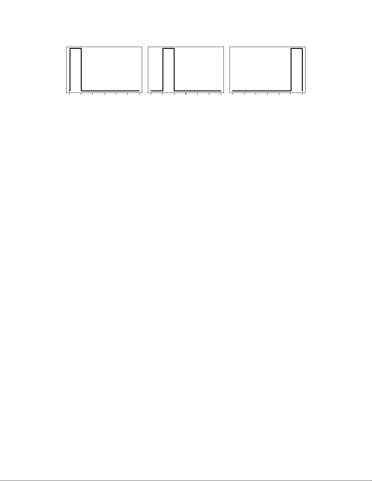
2. These distances ignore the underlying geometry of the space. To see this consider
Figure 1. In this figure we see three densities p
1
, p
2
, p
3
. It is easy to see that
R
|p
1
−p
2
| =
R
|p
1
− p
3
| =
R
|p
2
− p
3
| and similarly for the other distances. But our intuition tells
us that p
1
and p
2
are close together. We shall see that this is captured by Wasserstein
distance.
1
−3 −2 −1 0 1 2 3 −3 −2 −1 0 1 2 3 −3 −2 −1 0 1 2 3
Figure 1: Three densities p
1
, p
2
, p
3
. Each pair has the same distance in L
1
, L
2
, Hellinger
etc. But in Wasserstein distance, p
1
and p
2
are close.
3. When we average different objects — such as distributions or images — we would like
to make sure that we get back a similar object. The top plot in Figure 2 shows some
distributions, each of which is uniform on a circle. The bottom left plot shows the
Euclidean average of the distributions which is just a gray mess. The bottom right
shows the Wasserstein barycenter (which we will define later) which is a much better
summary of the set of images.
4. When we compute the usual distance between two distributions, we get a number but
we don’t get any qualitative information about why the distributions differ. But with
the Wasserstein distance we also get a map that shows us how we have to move the
mass of P to morph it into Q.
5. Suppose we want to create a path of distributions (a geodesic) P
t
that interpolates
between two distributions P
0
and P
1
. We would like the distributions P
t
to preserve
the basic structure of the distributions. Figure 5 shows an example. The top row
shows the path between P
0
and P
1
using Wasserstein distance. The bottom row shows
the path using L
2
distance. We see that the Wasserstein path does a better job of
preserving the structure.
6. Some of these distances are sensitive to small wiggles in the distribution. But we shall
see that the Wasserstein distance is insensitive to small wiggles. For example if P is
uniform on [0, 1] and Q has density 1+sin(2πkx) on [0, 1] then the Wasserstein distance
is O(1/k).
2 Optimal Transport
If T : R
d
→ R
d
then the the distribution of T (X) is called the push-forward of P , denoted
by T
#
P . In other words,
T
#
P (A) = P
{x : T (x) ∈ A
= P (T
−1
(A)).
2
Figure 2: Top: Some random circles. Bottom left: Euclidean average of the circles. Bottom
right: Wasserstein barycenter.
The Monge version of the optimal transport distance is
inf
T
Z
||x − T (x)||
p
dP (x)
where the infimum is over all T such that T
#
P = Q. Intuitively, this measures how far you
have to move the mass of P to turn it into Q. A minimizer T
∗
, if one exists, is called the
optimal transport map.
If P and Q both have densities than T
∗
exists. The map T
t
(x) = (1 −t)x + tT
∗
(x) gives the
path of a particle of mass at x. Also, P
t
= T
t#
P is the geodesic connecting P to Q.
But, the minimizer might not exist. Consider P = δ
0
and Q = (1/2)δ
−1
+ (1/2)δ
1
where
δ
a
. In this case, there is no map T such that T
#
P = Q. This leads us to the Kantorovich
formulation where we allow the mass at x to be split and move to more than one location.
Let J(P, Q) denote all joint distributions J for (X, Y ) that have marginals P and Q. In
other words, T
X#
J = P and T
Y #
J = Q where T
X
(x, y) = x and T
Y
(x, y) = y. Figure 4
shows an example of a joint distribution with two given marginal distributions. Then the
Kantorovich, or Wasserstein, distance is
W
p
(P, Q) =
inf
J∈J (P,Q)
Z
||x − y||
p
dJ(x, y)
1/p
3
剩余12页未读,继续阅读
Pearacle
- 粉丝: 0
- 资源: 1
上传资源 快速赚钱
- 我的内容管理 收起
- 我的资源 快来上传第一个资源
- 我的收益 登录查看自己的收益
- 我的积分 登录查看自己的积分
- 我的C币 登录后查看C币余额
- 我的收藏
- 我的下载
- 下载帮助
会员权益专享
最新资源
- c++校园超市商品信息管理系统课程设计说明书(含源代码) (2).pdf
- 建筑供配电系统相关课件.pptx
- 企业管理规章制度及管理模式.doc
- vb打开摄像头.doc
- 云计算-可信计算中认证协议改进方案.pdf
- [详细完整版]单片机编程4.ppt
- c语言常用算法.pdf
- c++经典程序代码大全.pdf
- 单片机数字时钟资料.doc
- 11项目管理前沿1.0.pptx
- 基于ssm的“魅力”繁峙宣传网站的设计与实现论文.doc
- 智慧交通综合解决方案.pptx
- 建筑防潮设计-PowerPointPresentati.pptx
- SPC统计过程控制程序.pptx
- SPC统计方法基础知识.pptx
- MW全能培训汽轮机调节保安系统PPT教学课件.pptx
资源上传下载、课程学习等过程中有任何疑问或建议,欢迎提出宝贵意见哦~我们会及时处理!
点击此处反馈
安全验证
文档复制为VIP权益,开通VIP直接复制
信息提交成功
评论0