过度参数化机器学习：理论与泛化能力

需积分: 0 117 浏览量更新于2023-04-28 1 收藏 2.03MB PDF 举报

“《过参数化机器学习理论》综述论文探讨了近年来机器学习领域的重大进展，特别是关于过参数化模型如何在实践中展现出优秀的泛化能力，这一现象挑战了传统的偏差-方差权衡理论，并揭示了双下降现象。” 本文主要关注的是机器学习中的一个核心议题：过参数化模型的泛化性能。过参数化指的是模型的复杂度远超训练数据的规模，理论上这样的模型会过度拟合训练数据，导致在新数据上的表现不佳。然而，实际情况却并非如此，许多过参数化的模型，包括线性模型和深度神经网络，即便在插值训练数据的情况下，也能在测试数据上表现出良好的泛化能力。传统的机器学习理论基于偏差-方差权衡的概念，认为模型的复杂度应该适中，以平衡训练数据的拟合程度（偏差）和对噪声的敏感性（方差）。然而，过参数化模型的泛化能力打破了这一规则，引发了研究人员对这一经典理论的重新审视。文章中提到的“双下降现象”是一个关键发现，它表明随着模型复杂度的增加，模型的测试误差先降低后升高再降低，即在某一过度参数化阶段，模型的性能反而优于未过参数化的最佳模型。为了理解这一现象，研究者需要发展新的理论框架。过参数化模型的学习机制可能涉及到如正则化、数据的内在结构、优化过程的性质以及模型的表示能力等多个方面。这些因素如何共同作用，使得模型能够在大量复杂度下避免过拟合并实现泛化，是当前理论研究的重要课题。此外，论文可能还涵盖了训练算法的影响，如随机梯度下降(SGD)在处理过参数化模型时的特殊行为，以及如何通过调整学习率、批次大小等参数来优化模型的泛化性能。研究者可能还讨论了在实际应用中，如何有效地利用过参数化模型，同时防止过拟合的策略，如早停法、dropout和数据增强等。《过参数化机器学习理论》综述论文旨在深入剖析过参数化模型背后的理论基础，揭示其泛化性能的秘密，这对于未来机器学习模型的设计和优化具有重要的指导意义。通过这样的研究，我们可以更好地理解和利用这些复杂的模型，推动机器学习技术的进一步发展。

where Σ

= C

and Λ

is a d × d real diagonal matrix. By Example 1, φ , U

x is the

p-dimensional feature vector where U

is a d ×p real matrix with orthonormal columns that extract

the features for the learning process. Consequently, φ ∼ N(0, Σ

) where Σ

= U

If the feature space for learning is based on DCT basis vectors (i.e., the columns of U

are the ﬁrst p

columns of C

), then the p × p input feature covariance matrix Σ

is diagonal; in fact, its diagonal

entries are exactly the ﬁrst p entries of the diagonal of the d × d data covariance matrix Λ

2.2. The double descent phenomenon

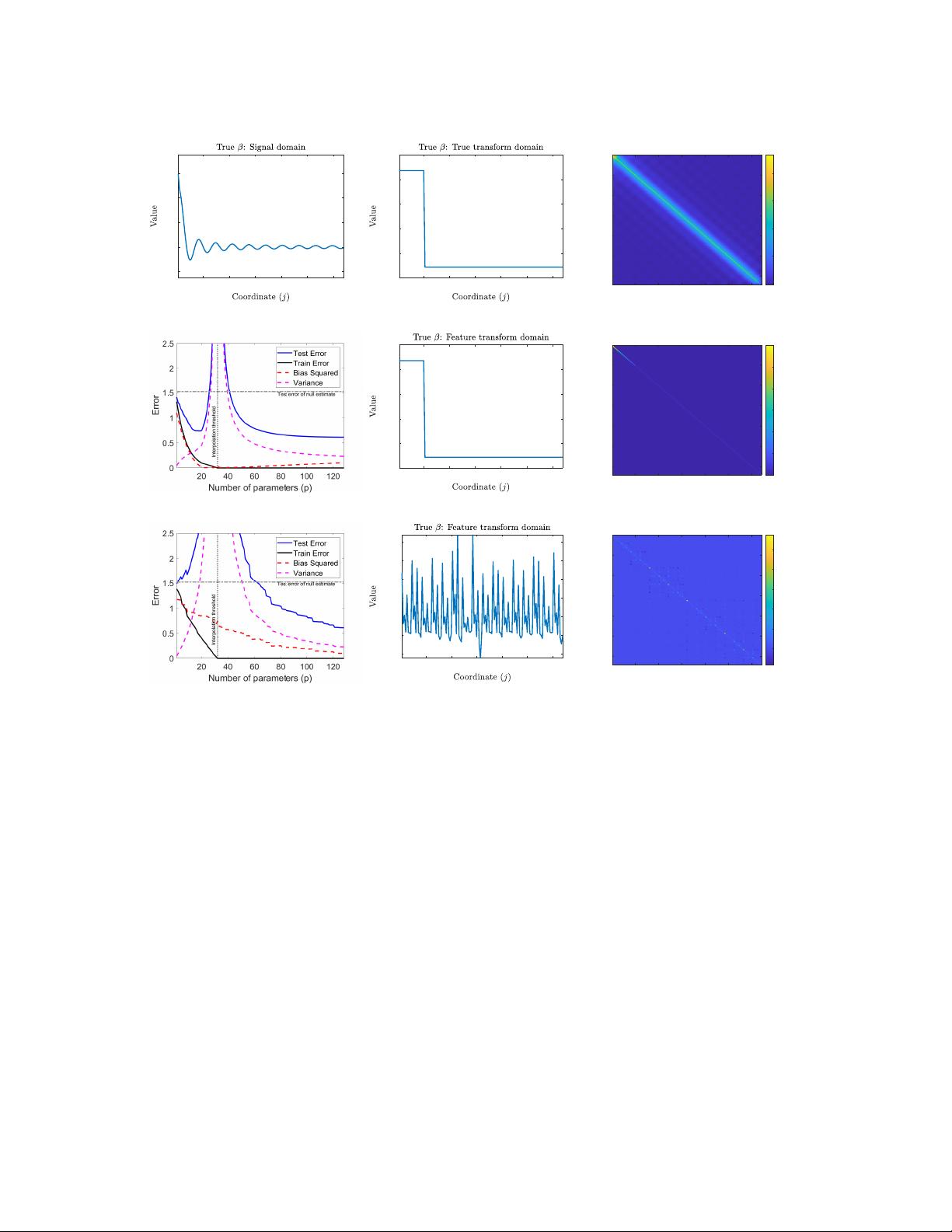
Figure 2 studies the relationship between model complexity (in number of parameters) and test

error induced by linear regression with a linear feature map (in line with Example 1). For both

experiments, we set d = 128 and n = 32, and vary the number of parameters p to be between 1

and d. We also consider β to be an approximately 20-sparse parameter vector such that the majority

of its energy is contained in the ﬁrst 20 discrete cosine transform (DCT) features (see Figure 2(b)

for an illustration). The input data covariance matrix Σ

is also considered to be anisotropic, as

pictured in the heatmap of its values in Figure 2(c).

We consider two choices of linear feature maps, i.e., two choices of orthonormal bases {u

}

j=1

the discrete cosine transform (DCT) basis and the Hadamard basis. In the ﬁrst case of DCT features,

the model is well-speciﬁed for p = d and the bulk of the optimal model ﬁt will involve the ﬁrst 20

features as a consequence of the approximate sparsity of the true parameter β in the DCT basis (see

Figure 2(e)). As a consequence of this alignment, the feature covariance matrix, Σ

, is diagonal

and its entries constitute the ﬁrst p entries of the diagonalized form of the data covariance matrix,

denoted by Λ

. The ensuing spiked covariance structure is depicted in Figure 2(f). Figure 2(d)

plots the test error as a function of the number of parameters, p, in the model and shows a counter-

intuitive relationship. When p < n = 32, we obtain non-zero training error and observe the classic

bias-variance tradeoff. When p > n, we are able to perfectly interpolate the training data (with

the minimum `

-norm solution). Although interpolation of noise is traditionally associated with

overﬁtting, here we observe that the test error monotonically decays with the number of parameters

p! This is a manifestation of the double descent phenomenon in an elementary example inspired by

signal processing perspectives.

The second choice of the Hadamard basis also gives rise to a double descent behavior, but is

quite different both qualitatively and quantitatively. The feature space utilized for learning (the

Hadamard basis) is fundamentally mismatched to the feature space in which the original parameter

vector β is sparse (the DCT basis). Consequently, as seen in Figure 2(h), the energy of the true

parameter vector β is spread over the d Hadamard features in an unorganized manner. Moreover,

the covariance matrix of Hadamard features, depicted as a heat-map in Figure 2(i), is signiﬁcantly

more correlated and dispersed in its structure. Figure 2(g) displays a stronger beneﬁt of overparam-

eterization in this model owing to the increased model misspeciﬁcation arising from the choice of

Hadamard feature map. Unlike in the well-speciﬁed case of DCT features, the overparameterized

regime signiﬁcantly dominates the underparameterized regime in terms of test performance.

Finally, the results in Fig. 3 correspond to β that its components are shown in Fig. 3(a) and its

DCT-domain representation is presented in Fig. 3(b). The majority of β’s energy is in a mid-range

“feature band” that includes the 18 DCT features at coordinates j = 21, . . . , 38; in addition, there

are two more high-energy features in coordinates j = 1, 2, and the remaining coordinates are of low

energy (see Fig. 3(b)). The input covariance matrix Σ

, presented in Fig. 3(c), is the same as before

剩余47页未读，继续阅读

syp_net

粉丝: 158
资源: 1187

过度参数化机器学习：理论与泛化能力

机器学习论文综述：NLP与资源不足问题研究

三角网格参数化综述：保性质与未来趋势

大规模机器学习优化方法综述：SGD挑战与未来趋势

《深度学习理论进展》综述论文

深度学习理论与架构最新进展综述论文

深度主动学习综述论文

深度学习轻量化目标检测综述（论文及思维导图）

最新《计算机视觉持续学习进展》综述论文

深度强化学习的论文综述

机器学习Lasso回归重要论文和Matlab代码

最新资源