matlab最优化编程方法_matlab最优化程序

matlab

向量化

需积分: 9 196 浏览量更新于2023-05-28 评论 1 收藏 234KB PDF 举报

身份认证购VIP最低享 7 折!

领优惠券(最高得80元）

资源详情

资源评论

资源推荐

DIFFERENTIAL GEOMETRY OF CURVES AND SURFACES

1. Curves in the Plane

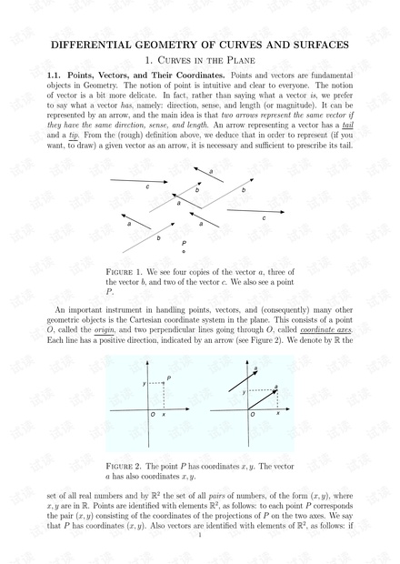
1.1. Points, Vec tors, and Their Coordinates. Points and vectors are fundamental

objects in Geometry. The notion of point is intuitive and clear to everyone. The notion

of vector is a bit more delicate. In fa ct, rather than saying what a vector is, we prefer

to say what a vector has , namely: direction, sense, and length (or magnitude). It can be

represented by an arrow, and the main idea is that two arrows represent the same vector if

they have the same direction, sense, and length. An arrow representing a vector has a tail

and a tip. From the (ro ugh) deﬁnition a bove, we deduce that in order to represent (if yo u

want, to draw) a given vector as an arrow, it is necessary and suﬃcient to prescribe its tail.

a a

Figure 1. We see four copies of the vector a, three of

the vector b, and two of the vector c. We a lso see a point

P .

An important instrument in handling points, vectors, and (consequently) many other

geometric objects is the Cartesian coordinate system in the plane. This consists of a point

O, called the origin, and two perpendicular lines going through O, called coordinate axes.

Each line has a positive direction, indicated by an arrow (see Figure 2). We denote by R the

O O

Figure 2. The point P has coordinates x, y. The vector

a has also coordinates x, y.

set of all real numbers and by R

the set of all pairs of numbers, of the form (x, y) , where

x, y are in R. Points are identiﬁed with elements R

, as follows: to each point P corresponds

the pair (x, y) consisting of the coordinates of the projections of P on the two axes. We say

that P has coordinates (x, y). Also vectors a re identiﬁed with elements of R

, as follows: if

a is a vector, we move its tail to the origin O, and we take the coordinates of its tip. We say

that a has coordinates (x, y). One of the ﬁrst advantag es of the coordinate system is that

we can use it to compute lengths, as follows. The distance between the points P

= (x

, y

)

and P

= (x

, y

) is

k =

− x

)

+ (y

− y

)

The length of the vector a = (x, y) is

kak =

+ y

In our course, R

will denote both the set of all points and the set of all vectors (in the

plane). It will always be possible to understand from the context if a certain object in R

a point or a vector.

1.2. Parametrized Curves. A good way of thinking of a curve is as the object which

describes the motion of a particle in the plane: at the time t, the particle is at the point in

the plane whose coordinates are (x(t), y(t)). We stress from the very beginning that what

we are interested in is not simply w h at the trajectory of the particle is, but ra t her how the

trajectory is r un. Now comes the exact deﬁnition.

Deﬁnition 1.2.1. A parametrized curve in the plane

is a diﬀerentiable f unction

α(t) = (x(t), y(t)),

where t satisﬁes a < t < b (possibly a and/or b can be ∞).

When we say that α(t) = (x(t), y(t)) is “diﬀerentiable” we mean that both x(t) and y(t)

have derivative of any order (we also say that they are C

∞

diﬀerentiable).

The standard notation for such an object is

α : (a, b) → R

where (a, b) is the open interval between a and b. As we already mentioned, it is importa nt

to distinguish between the curve α (the assignment which associates to any “time” t the

point (x(t), y(t)) on t he “t rajectory”) and the image of the function α (the “trajectory”).

The latter is called the trace

of the curve α.

Remark. Very of t en it is possible to describe the tra ce of a curve α : (a, b) → R

with

α(t) = (x(t), y(t)), by an equation of the form f(x, y) = 0, where f is a function of variables

x, y. If so, we say that

x = x(t), y = y(t)

are the parametric equations

(or explicit equations) of the curve and

f(x, y) = 0

is the implicit equation

of the curve. For example, the trace of the curve

x = 1 − 2t, y = 5t

is a straight line (see below). The same line can be describ ed by the implicit equation

5x + 2y = 5.

Also, the circle of radius 1 and centre 0 can be described as the trace of

x = cos t, y = sin t

It is worth mentioning that the domain of the function α is the interval a < t < b a nd the range is R

剩余19页未读，继续阅读

weixin_43102907

粉丝: 0
资源: 1

会员权益专享

matlab最优化编程方法

评论0

会员权益专享

最新资源

matlab最优化编程方法

评论0

使用Matlab余元编程，进行三自由度的非线性车辆动力学建模

Matlab最优化编程例子

matlab微电网优化调度

鸽群优化算法matlab

matlab gwo 优化svm回归预测

免疫优化配送算法 matlab

遗传算法优化matlab程序

轴向拉压等直杆变形matlab编程

鲸鱼优化多目标优化matlab代码

粒子群加速法pid matlab编程

lns算法matlab编程

小生境粒子群优化算法matlab

多目标优化算法 nsga-Ⅲ matlab

粒子群优化模糊控制matlab

基于matlab的综合能源系统多能流转换编程源码

python和matlab的相互转换

frank wolfe算法编程matlab

智能优化算法及其matlab实例（第2版）

lmi matlab 一些特殊的例子

基于matlab粒子群算法求解系统经济、环境运行目标调度优化matlab

会员权益专享

最新资源