没有合适的资源?快使用搜索试试~ 我知道了~
首页反卷积(卷积层的可视化)
反卷积(卷积层的可视化)
需积分: 50 1.9k 浏览量
更新于2023-05-25
评论 4
收藏 667KB PDF 举报
反卷积(Deconvolution)的概念第一次出现是Zeiler在2010年发表的论文Deconvolutional networks中,但是并没有指定反卷积这个名字,反卷积这个术语正式的使用是在其之后的工作中(Adaptive deconvolutional networks for mid and high level feature learning)。随着反卷积在神经网络可视化上的成功应用,其被越来越多的工作所采纳比如:场景分割、生成模型等。其中反卷积(Deconvolution)也有很多其他的叫法,比如:Transposed Convolution,Fractional Strided Convolution等等。
资源详情
资源评论
资源推荐

Workshop track - ICLR 2016
STACKED WHAT-WHERE AUTO-ENCODERS
Junbo Zhao, Michael Mathieu, Ross Goroshin, Yann LeCun
Courant Institute of Mathematical Sciences, New York University
719 Broadway, 12th Floor, New York, NY 10003
{junbo.zhao, mathieu, goroshin, yann}@cs.nyu.edu
ABSTRACT
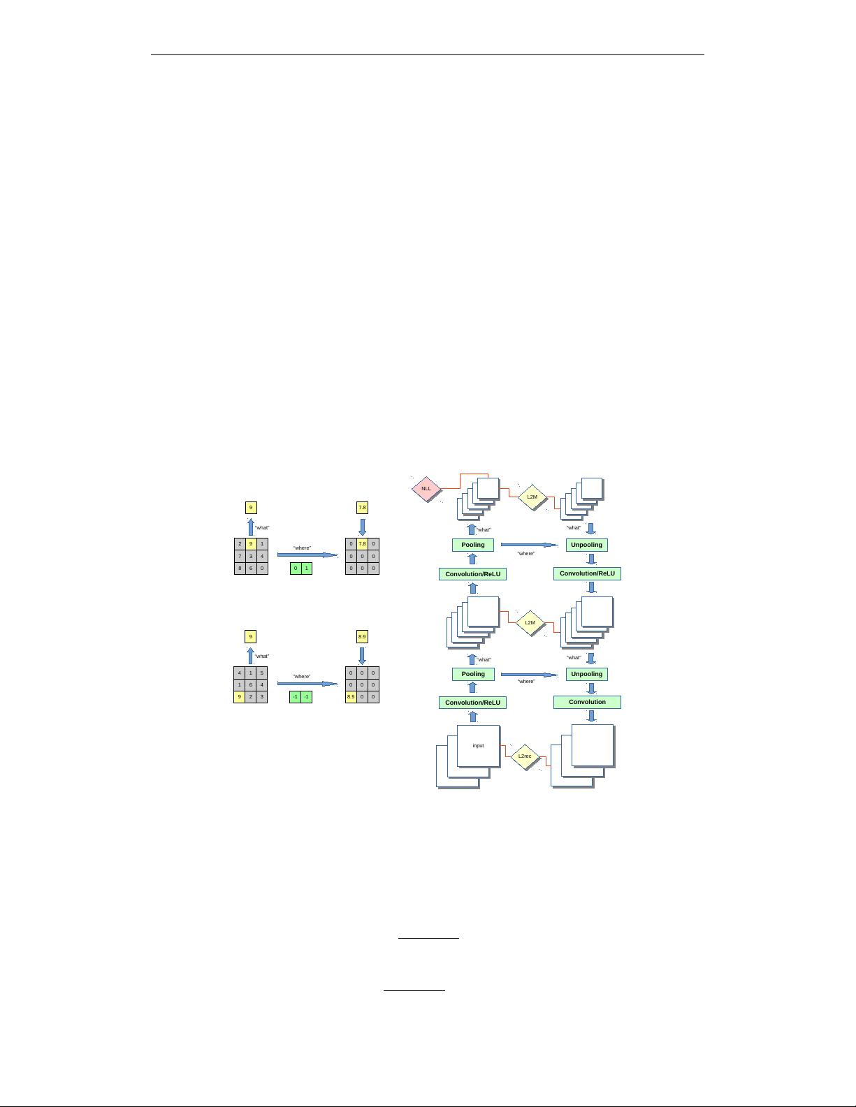
We present a novel architecture, the “stacked what-where auto-encoders”
(SWWAE), which integrates discriminative and generative pathways and provides
a unified approach to supervised, semi-supervised and unsupervised learning with-
out relying on sampling during training. An instantiation of SWWAE uses a con-
volutional net (Convnet) (LeCun et al. (1998)) to encode the input, and employs a
deconvolutional net (Deconvnet) (Zeiler et al. (2010)) to produce the reconstruc-
tion. The objective function includes reconstruction terms that induce the hidden
states in the Deconvnet to be similar to those of the Convnet. Each pooling layer
produces two sets of variables: the “what” which are fed to the next layer, and
its complementary variable “where” that are fed to the corresponding layer in the
generative decoder.
1 INTRODUCTION
A desirable property of learning models is the ability to be trained in supervised, unsupervised, or
semi-supervised mode with a single architecture and a single learning procedure. Another desirable
property is the ability to exploit the advantageous discriminative and generative models. A popular
approach is to pre-train auto-encoders in a layer-wise fashion, and subsequently fine-tune the entire
stack of encoders (the feed-forward pathway) in a supervised discriminative manner (Erhan et al.
(2010); Gregor & LeCun (2010); Henaff et al. (2011); Kavukcuoglu et al. (2009; 2008; 2010); Ran-
zato et al. (2007); Ranzato & LeCun (2007)). This approach fails to provide a unified mechanism
to unsupervised and supervised learning. Another approach, that provides a unified framework for
all three training modalities, is the deep boltzmann machine (DBM) model (Hinton et al. (2006);
Larochelle & Bengio (2008)). Each layer in a DBM is an restricted boltzmann machine (RBM),
which can be seen as a kind of auto-encoder. Deep RBMs have all the desirable properties, however
they exhibit poor convergence and mixing properties ultimately due to the reliance on sampling dur-
ing training. The main issue with stacked auto-encoders is asymmetry. The mapping implemented
by the feed-forward pathway is often many-to-one, for example mapping images to invariant features
or to class labels. Conversely, the mapping implemented by the feed-back (generative) pathway is
one-to-many, e.g. mapping class labels to image reconstructions. The common way to deal with this
is to view the reconstruction mapping as probabilistic. This is the approach of RBMs and DBMs:
the missing information that is required to generate an image from a category label is dreamed up
by sampling. This sampling approach can lead to interesting visualizations, but is impractical for
training large scale networks because it tends to produce highly noisy gradients.
If the mapping from input to output of the feed-forward pathway were one-to-one, the mappings
in both directions would be well-defined functions and there would be no need for sampling while
reconstructing. But if the internal representations are to possess good invariance properties, it is
desirable that the mapping from one layer to the next be many-to-one. For example, in a Convnet,
invariance is achieved through layers of max-pooling and subsampling.
Our model attempts to satisfy two objectives: (i)-to learn a factorized representation that encodes
invariance and equivariance, (ii)-we want to leverage both labeled and unlabeled data to learn this
representation in a unified framework. The main idea of the approach we propose here is very
simple: whenever a layer implements a many-to-one mapping, we compute a set of complemen-
tary variables that enable reconstruction. A schematic of our model is depicted in figure 1 (b). In
the max-pooling layers of Convnets, we view the position of the max-pooling “switches” as the
1
arXiv:1506.02351v8 [stat.ML] 14 Feb 2016

Workshop track - ICLR 2016
complementary information necessary for reconstruction. The model we proposed consists of a
feed-forward Convnet, coupled with a feed-back Deconvnet. Each stage in this architecture is what
we call a “what-where auto-encoder”. The encoder is a convolutional layer with ReLU followed by
a max-pooling layer. The output of the max-pooling is the “what” variable, which is fed to the next
layer. The complementary variables are the max-pooling “switch” positions, which can be seen as
the “where” variables. The “what” variables inform the next layer about the content with incomplete
information about position, while the “where” variables inform the corresponding feed-back decoder
about where interesting (dominant) features are located. The feed-back (generative) decoder recon-
structs the input by “unpooling” the “what” using the “where”, and running the result through a
reconstructing convolutional layer. Such “what-where” convolutional auto-encoders can be stacked
and trained jointly without requiring alternate optimization (Zeiler et al. (2010)). The reconstruction
penalty at each layer constrains the hidden states of the feed-back pathway to be close to the hidden
states of the feed-forward pathway. The system can be trained in purely supervised manner: the
bottom input of the feed-forward pathway is given the input, the top layer of the feed-back pathway
is given the desired output, and the weights of the decoders are updated to minimize the sum of
the reconstruction costs. If only the top-level cost is used, the model reverts to purely supervised
backprop. If the hidden layer reconstruction costs are used, the model can be seen as supervised
with a reconstruction regularization. In unsupervised mode, the top-layer label output is left un-
constrained, and simply copied from the output of the feed-forward pathway. The model becomes
a stacked convolutional auto-encoder. As with boltzmann machines (BM), the underlying learn-
ing algorithm doesn’t change between the supervised and unsupervised modes and we can switch
between different learning modalities by clamping or unclamping certain variables. Our model is
particularly suitable when one is faced with a large amount of unlabeled data and a relatively small
amount of labeled data. The fact that no sampling (or contrastive divergence method) is required
gives the model good scaling properties; it is essentially just backprop in a particular architecture.
2 RELATED WORK
The idea of “what” and “where” has been defined previously in different ways. One related method
was proposed known as “transforming auto-encoders” (Hinton et al. (2011)), in which “capsule”
units were introduced. In that work, two sets of variables are trained to encapsulate “invariance” and
“equivariance” respectively, by providing the parameters of particular transformation states to the
network. Our work is carried out in a more unsupervised fashion in that it doesn’t require the true
latent state while still being able to encode similar representations within the “what” and “where”.
Switches information is also made use of by some visualization work such as Zeiler et al. (2010),
while such work only has a generative pass and merely uses a feed-forward pass as an initialization
step.
Similar definitions have been applied to learn invariant features (Gregor & LeCun (2010); Henaff
et al. (2011); Kavukcuoglu et al. (2009; 2008; 2010); Ranzato et al. (2007); Ranzato & LeCun
(2007); Makhzani & Frey (2014); Masci et al. (2011)). Among them, most works merely shed light
to unsupervised feature learning and therefore failed to unify different learning modalities. Another
relevant hierarchical architecture is proposed in (Ranzato et al. (2007); Ranzato & LeCun (2007)),
however, because this architecture is trained in a layer-wise greedy manner, its performance is not
competitive with jointly trained models.
In terms of joint loss minimization and semi-supervised learning, our work can be linked to Weston
et al. (2012) and Ranzato & Szummer (2008), with the main advantage being the easiness to extend a
Convnet with a Deconvnet and thereby enabling the utilization of unlabeled data. Paine et al. (2014)
has analyzed the regularization effect with similar architectures in a layer-wise fashion.
One recent work (Rasmus et al. (2015b), Rasmus et al. (2015a)) has been proposed to adopt deep
auto-encoders to support supervised learning in which completely different strategy is employed to
harness the lateral connection between same stage encoder-decoder pairs, however. In that work,
decoders receive the entire pre-pooled activation state from the encoder, whereas decoders from
SWWAE only receive the “where” state from the corresponding encoder stages. Further, due to a
lack of unpooling mechanism incorporated in the Ladder networks, it is restricted to only reconstruct
the top layer within generative pathway (Γ model), which looses the ”ladder” structure. By contrast,
SWWAE doesn’t suffer from such necessity.
2

Workshop track - ICLR 2016
3 MODEL ARCHITECTURE
We consider the loss function of SWWAE depicted in figure 1(b) composed of three parts:
L = L
NLL
+ λ
L2rec
L
L2rec
+ λ
L2M
L
L2M
, (1)
where L
NLL
is the discriminative loss, L
L2rec
is the reconstruction loss at the input level and L
L2M
charges intermediate reconstruction terms. λ’s weight the losses against each other.
Pooling layers in the encoder split information into “what” and “where” components, depicted in fig-
ure 1(a), that “what” is essentially max and “where” carries argmax, i.e., the switches of maximally
activation defined under local coordinate frame over each pooling region. The “what” component is
fed upward through the encoder, while the “where” is fed through lateral connections to the same
stage in the feed-back decoding pathway. The decoder uses convolution and “unpooling” opera-
tions to approximately invert the output of the encoder and reproduce the input, shown in figure 1.
The unpooling layers use the “where” variables to unpool the feature maps by placing the “what”
into the positions indicated the preserved switches. We use negative log-likelihood (NLL) loss for
classification and L2 loss for reconstructions; e.g,
L
L2rec
= kx − ˜xk
2
, L
L2M
= kx
m
− ˜x
m
k
2
, (2)
where L
L2rec
denotes the reconstruction loss at input-level and L
L2M
denotes the middle recon-
struction loss. In our notation, x represents the input (no subscripts) and x
i
(with subscripts) repre-
sent the feature map activations of the Convnet, respectively. Similarly, ˜x and ˜x
m
are the input and
activations of the Deconvnet, respectively. The entire model architecture is shown in figure 1(b).
Notice in the following, we may use L
L2∗
to represent the weighted sum of L
L2rec
and L
L2M
.
input
input
“what”
“what”
“where”
Pooling
Unpooling
L2M
L2M
L2rec
L2rec
L2M
L2M
NLL
NLL
“what”
“what”
“where”
Pooling
Unpooling
4 1 5
1 6 4
9 2 3
0 0 0
0 0 0
8.9 0 0
“where”
“what”
9
-1 -1
8.9
2 9 1
7 3 4
8 6 0
0 7.8 0
0 0 0
0 0 0
“where”
“what”
9
0 1
7.8
Convolution/ReLU
Convolution
Convolution/ReLU
Convolution/ReLU
Figure 1: Left (a): pooling-unpooling. Right (b): model architecture. For brevity, fully-connected
layers are omitted in this figure.
3.1 SOFT VERSION “WHAT” AND “WHERE”
Recently, Goroshin et al. (2015) introduces a soft version of max and argmax operators within each
pooling region:
m
k
=
X
N
k
z(x, y)
e
βz(x,y)
P
N
k
e
βz(x,y)
≈ max
N
k
z(x, y) (3)
p
k
=
X
N
k
x
y
e
βz(x,y)
P
N
k
e
βz(x,y)
≈ arg max
N
k
z(x, y), (4)
3
剩余11页未读,继续阅读


安全验证
文档复制为VIP权益,开通VIP直接复制

评论0