没有合适的资源?快使用搜索试试~ 我知道了~
首页LIFBASE帮助文件
资源详情
资源评论
资源推荐

LIFBASE (version 1.9)
http://www.sri.com/cem/lifbase
DATABASE AND SPECTRAL SIMULATION
for OH A-X, OD A-X,
NO A-X, B-X, C-X, D-X
CH A-X, B-X, C-X
CN B-X, N
2
+
B-X,
SiH A-X and CF A-X
by Jorge Luque and David R. Crosley
SRI International
SRI report No. MP 99-009 (1999)

1
LIFBASE: Database and spectral simulation program.
1. Goal:
This program has been designed to compile all the information available from
transition probability calculations on the diatomic molecules OH, OD, CH and NO. These
molecules are important in a wide variety of research fields, from basic studies in
chemical dynamics to applied works in combustion. This report complements work to
several manuscripts on spectroscopy of these molecules by the same authors.
1-4,23,32
The output of this program furnishes Einstein emission and absorption
coefficients, radiative lifetimes, transition probabilities, frequencies and Hönl-London
factors for many bands of OH (A-X), OD (A-X), CH (A-X, B-X, C-X), NO (A-X, D-X),etc.
Also, spectral simulation in these electronic systems can be done, including the
possibility of modifying many parameters interactively.
Wavelength (Å)
3050 3100 3150 3200 3250
Intensity
CH C-X(0,0)
CH C-X(1,1)
OH A-X
OH A-X
Observed emission
Simulation
R
P
Q(0,0)
Q(1,1)
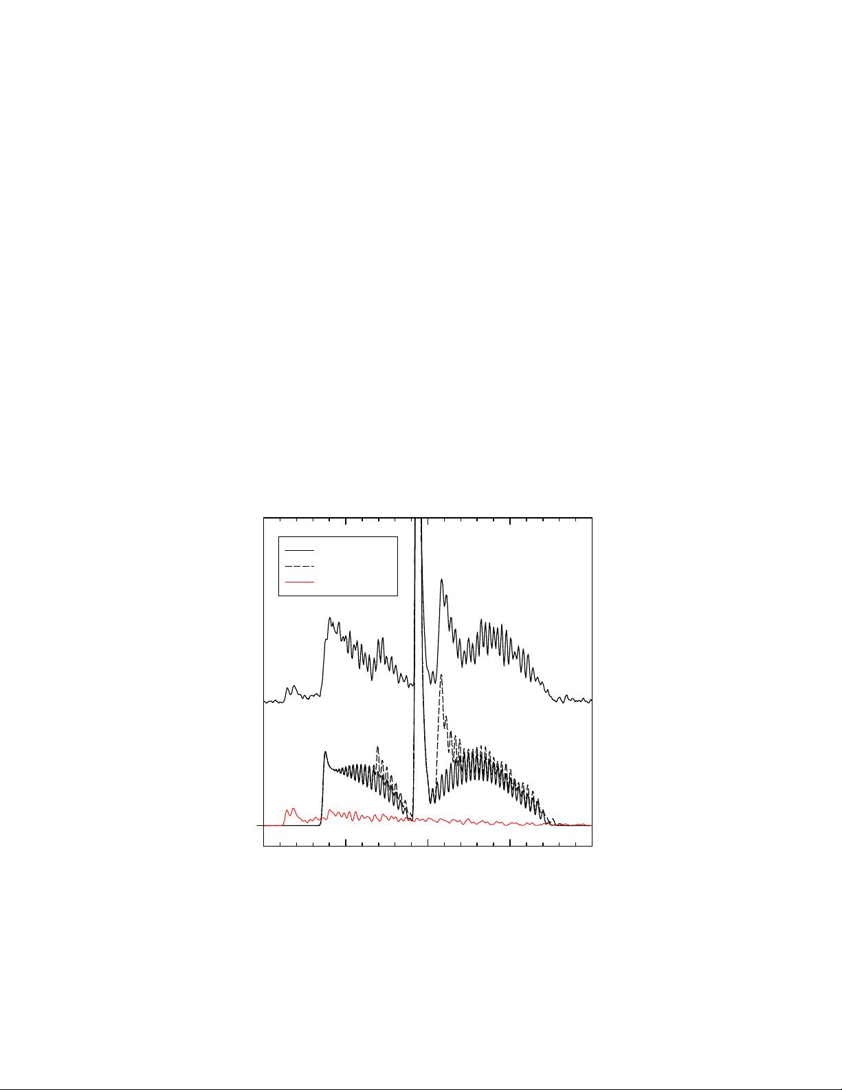
Figure 1. Example of optical emission spectral simulation of CH C-X in a plasma dc-reactor
(Vibrational and rotational temperatures = 5500 K)

2
2. Program description:
2.1. Database:
When the program initially starts, it provides a table with the quantity calculated
during the last execution. The menu allows the user to change the electronic band and
the spectroscopic quantities calculated.
a) The
emission coefficients
between upper levels v’,J’ and a lower levels v”,J”
are calculated according to Schadee
5
, by the expression (s
-1
):
()
A
g
g
h
S
J
p
vJ
vJ
e
e
J
J
vJ
vJ
vJ
vJ
""
''
'
"
"
'
""
''
""
''
'
=
+
64
321
4
3
π
υ
the electronic degeneracy is g
e
= (2-
δ
o,
Λ
)(2S+1), 2S+1 is the state spin multiplicity
and
δ
o,
Λ
=1 for
Σ
states and 0 for all the others.
S
is the Honl-London factor,
p
is the
transition probability and
υ
is the transition frequency (cm
-1
).
b) The
absorption coefficients
are calculated by the expression:
()
B
c
h
J
J
A
vJ
vJ
vJ
vJ
vJ
vJ
''
""
""
''
""
''
'
"
=
+
+
2
3
8
21
21
πυ
The stimulated emission coefficients are
B
J
J
B
vJ
vJ
vJ
vJ
""
''
''
""
"
'
=
+
+
21
21
The units (m
2
s
-1
J
-1
) are convenient in LIF applications and can be converted to
the common (m
3
s
-2
J
-1
) via multiplying by the speed of light
c
. Oscillator strengths are
also calculated and displayed.
The absorption and emission coefficients have the lambda-doubling resolved for
Π
and
∆
states, and the corresponding populations must therefore be computed per
lambda-doubled level as well. This is an important detail to avoid errors of factor of two
when the
Π
->
Σ
transitions are used to determine absolute number densities.

3
c)
Transition probabilities
: They have been previously calculated and are kept
in the data base files. Transition probabilities are the integrals of the rovibrational
wavefunctions of the upper and lower states together with the electronic transition
moment:
prRrrdr
vJ
vJ
vJevJ
""
''
'' ""
() () ()
=
−∞
∞
∫
ΨΨ
2
The wavefunctions are computed from RKR potential curves, and R
e
(r) is the
electronic transition moment. See tables I -II for more detailed information on the input
data for the calculations. Rotational wavefunctions are not included for the NO A-X
(disk version), B-X, D-X, N
2
+
B-X and CN B-X transition probabilities, those files can be
obtained upon request.
The electronic transition moment can be obtained by ab initio methods, or by
experimentally based techinques, like branching intensitiy ratios combined with either
radiative lifetimes or absorption oscillator strenghts. LIFBASE includes experimentally
optimized transition moments or experimentally validated ab initio calculations, see
references 1-3, 32 and 37.
Figure 2.
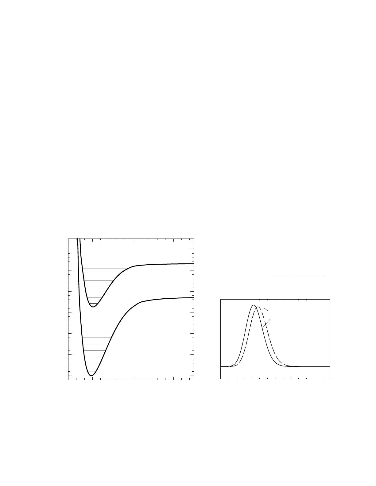
Calculation of rovibrational wavefunctions from RKR potential curves. Left: OH
A and X states potential curves from RKR calculations with input data from tables I and II. Right:
Effect of rotational centrifugal barrier on the wavefunctions.
Internuclear Distance r (Å)
123
Energy (cm
-1
)
0
10000
20000
30000
40000
50000
60000
O (
1
D) + H (
2
S)
O (
3
P) + H (
2
S)
X
2
Π
A
2
Σ
+
0
1
2
3
4
5
6
0
1
2
3
4
Internuclear Distance r (Å)
1.0 1.5 2.0
22
2
)1(
8
)()(
r
JJh
rVrV
eff
+
⋅+=
µπ
The wavefunctions vary with
rotational quantum number
because of the effective potential :
OH A-X POTENTIAL CURVES
OH A v'=0 N'=20
OH A v'=0 N'=0

4
d)
Frequencies
: These are calculated from expressions derived from the
corresponding Hamiltonians (most cases this is the N-formalism, known as Brown’s
Hamiltonian
6
), so the accuracy of line-positions may be limited in some cases. The units
are cm
-1
, Å (vacuum) or Å (air).
The nomenclature of the branches is either Hund’s case
a
or
b
. The program
supports both cases switching with the “J” and “N” keys. In Hund’s case
b
the name of
the rotational branches is given by
∆
N =N’-N” rather than
∆
J (N’, excited state; N”,
ground state):
Case a:
∆
N
∆
J
F’F”
(J”) Case b:
∆
J
∆
N
F’F”
(N”)
and
∆
N or
∆
J =-2,-1,0,1,2
!
O,P,Q,R,S
The rotational lines are assigned by N quantum numbers in Hund’s case
b
, this
notation can be changed to J numbers, Hund’s case
a
. The lines with ground state
terms from the spin-orbit F
1
: J=N+1/2 and from F
2
: J=N-1/2. For example:
NO A-X
R
R
11
(N”=1) [case b] ->
R
R
11
(J”=1.5) = R
1
(1.5) [case a]
e) Line-strengths or
Hönl-London factors
: Following the analytical expressions
by Kovacs
7
and Earls
8
. The normalization is as suggested by Whiting
9
:
SSJ
J
J
J
"
'
"
,' "
()(')(')
∑
=− + +
+
22121
0
δ
ΛΛ
f)
Lifetimes
are calculated by:
τ
vJ
e
vJ
vJ
vJ
g
A
''
'
""
''
""
=
∑
and normalized to the chosen experimental
τ
v’=0
(in ns).
g)
Predissociation
rates (Kp
v’J’
) and
quenching
(Kq
v’J’
) rate coefficients can be
included in the calculation of fluorescence quantum yields through user provided files.
The program comes with the most accurate predissociation rates known, and the
quenching set to zero. The column title to identify radiative lifetime is
t
r
collision free
lifetime is
t
p
, and the fluorescence quantum yield including quenching is
Y
f
.
Also, one can choose to study a particular vibrational band and obtain a
complete table with the main and the satellite branches. Finally, the program is able to
print or create a file with the selections made.
剩余21页未读,继续阅读


安全验证
文档复制为VIP权益,开通VIP直接复制

评论0