没有合适的资源?快使用搜索试试~ 我知道了~
首页Understanding Automotive Electronics 8th - Appendix B
Understanding Automotive Electronics 8th - Appendix B
需积分: 10 13 下载量 94 浏览量
更新于2023-05-26
评论
收藏 547KB PDF 举报
Understanding Automotive Electronics 8th Appendix B - Discrete Time Systems Theory
资源详情
资源评论
资源推荐
APPENDIX
DISCRETE TIME SYSTEMS THEORY
B
As explained in Appendix A, automotive electronic control and instrumentation systems (as well as
virtually all other electrical systems) are implemented with digital electronics as at least some com-
ponent or subsystem. Digital controllers and/or signal processing subsystems incorporate one or more
microprocessors or microcontrollers, each having a stored program to run the system. Su ch systems are
fundamentally discrete time systems.
However, automotive electronic systems also incorporate analog or continuous time components
(e.g., sensors and actuators). In order for the digital subsystem to perform its intended operation, it
has, for its input/output variables, numerical values of the continuous input/output at discrete times
(t
k
where k ¼1, 2,…). The time between successive input/output values must be sufficient for the digital
system to perform all operations on the input to gener ate an output.
Although it is not necessary, most discrete time systems use periodic times to represent input/out-
put; that is, the kth discrete time is given by
t
k
¼ kT
s
k ¼ 1,2,3,⋯
where T
s
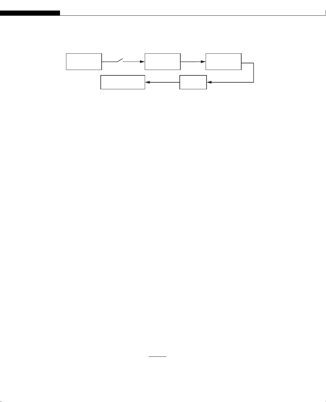
is the sample period. The configuration for a discrete time system with an embedded digital
system and an analog destination component is depicted in Fig. B.1.
In this figure, the source has a continuous time electrical signal v(t) that could, for example, be a
sensor output. The interface electronics-labeled A/D converter (which is modeled later in this appendix)
generates a sequence of numerical values called samples at each discrete time or “sample period” t
k
:
v
k
¼ v t
k
ðÞ
These samples must be in a format that can be input to the digital system. The input to the digital system
at t
k
is denoted x
k
, which is a digital (N bit) numerical value equal to v
k
; that is, the sampled variable v
k
becomes a binary number x
k
. The digital system generates an output y
n
associated with input sample x
n
(as well as previous samples depending on the operations performed). Although the destination
component might be a display device that can display the desired output numerical value, it may also
be an actuator requiring a continuous time electrical signal y(t). We assume here that the destination
component (e.g., a display or actuator) requires a continuous time electrical input. This continuous time
electrical signal is generated from the output y
n
via an output interface D/A converter. A system that is
partly continuous time along with one or more sampling operations is called a sampled data system or a
discrete time system.
It is important whe n explaining such systems for either design or performance analysis to develop
appropriate models for mixed continuous and discrete time systems. For the purpose of developing
such models, it is helpful to discuss initially only linear, time-invariant systems. In chapters that are
641
concerned with specific auto motive systems, we deal with nonlinearities as required to explain the
particular system.
As shown in the Appe ndix A, a linear time-invariant continuous time system is characterized by an
nth order differential equation with constant coefficients. The linear time-invariant discrete time sys-
tem is characterized by a model in the format of difference equations. One commonly used model for
calculating the output y
n
of a discrete time system is in the form of a recursive model:
y
n
¼
X
K
k¼0
a
k
x
nk
X
L
‘¼1
b
‘
y
n‘
(B.1)
The dynamic response of such a system is determined by the coefficients a
k
and b
‘
.
It is shown in Appendix A that a continuous time system is usefully characterized by its transfer
system (H(s)), whi ch is obtained from the Laplace transforms of its input and output. A similar pro-
cedure is very useful for conducting performance analysis or design of a discrete time digital system.
For a discrete time system, the transform of a sequence x
n
that is analogous to the Laplace transf orm
for a continuous time system is the Z-transform X(z) defined by
XzðÞ¼Z x
n
ðÞ
XzðÞ¼
X
∞
n¼∞
x
n
z
n
(B.2)
We illustrate with an example in which x
n
is defined as
x
n
¼ c
n
n 0
¼ 0 n 0
(B.3)
The Z-transform is given by
XzðÞ¼
X
∞
n¼0
c
n
z
n
¼
X
∞
n¼0
cz
1
n
(B.4)
where z ¼ complex variable analogous to s for the Laplace transform. This latter sum is a geometric
series that conver ges if cz
1
1or z
jj
c
jj
to the closed form result
XzðÞ¼
1
1 cz
1
z
jj
c
jj
(B.5)
There are several important elementary properties of the Z-transform that are important in the analysis
of discrete time digital systems that are summarized without proof below:
v(t)
y(t)
A/D
D/A
Output interface
Digital systems
x
k
y
k
v(t
k
)
Sampler
Source variable
Destination
component
T
FIG. B.1 Discrete time system configuration.
642 APPENDIX B DISCRETE TIME SYSTEMS THEORY
1. Linearity:
Z ax
n
+ by
n
½
¼ aX z
ðÞ
+ bY z
ðÞ
(B.6)
2. Time shift by an integer k
Z x
n + k
½
¼ z
k
Xz
ðÞ
(B.7)
3. Convolution: let
W
n
¼
X
∞
k¼∞
x
k
y
nk
¼
X
∞
n¼∞
x
nk
y
k
(B.8)
then
W(z) ¼X(z)Y(z)
As in the case of a continuous time system for which the inverse Laplace transform can be found,
there is an inverse Z-transform of X(z) yielding the sequence {x
n
}denoted as Z
1
XzðÞ½¼x
n
fg
, which
is given by the following contour integral in the complex z-plane:
x
n
¼
1
2πj
þ
C
XzðÞz
n
dz
z
(B.9)
where the contour C is chosen in a region of the complex z-plane for which the series converges.
It is assumed that Y(z) is the Z-transform of a sequence y
n
that is bounded as n !∞. In this case
(which is the case of practical significance in any automotive electronic system), the unit circle in the
complex z-plane (i.e., jzj¼1) forms the boundary of the region of convergence of Y(z). All poles of Y(z)
lie inside the unit circle, and Y(z) is analytic for jzj> 1. The inverse Z-transform of Y(z) is a single-sided
sequence {y
n
} where
y
n
¼ 0 n < 0
In this case (of practical interest), the contour C is the unit circle (i.e., C !jzj¼1).
In practice, the inverse Z-transform of a function of z (e.g., Y(z)) is normally computed from a par-
tial fraction expansion of Y(z) about its poles z
k
:
YzðÞ¼
X
n
j¼1
a
j
z z
j
¼
X
n
j¼1
a
j
z
1
1 z
j
z
1
(B.10)
where a
j
¼ residue at pole z
j.
The residue theorem was explained in Appendix A and applies equally to the partial fraction ex-
pansion of functions of complex variable z.
Each of these terms can be rewritten in the form of a Taylor series for each pole provided jzj> jz
j
j:
a
j
z
1
1 z
j
z
1
¼ a
j
X
∞
m¼0
z
j
m
z
m +1ðÞ
j ¼ 1, 2, ⋯,n (B.11)
Replacing the summation index m with k 1 and beginning the series sum with k ¼ 1 yield an expres-
sion for each partial fraction of the same form as Y(z). Combining terms of like power yields the
following expression for Y(z):
643APPENDIX B DISCRETE TIME SYSTEMS THEORY
YzðÞ¼
X
∞
k¼1
X
n
j¼1
a
j
z
j
k1
"#
z
k
(B.12)
Comparing like powers of z of Eq. (B.12) with the definition of Y(z) yields the inverse Z-transform of
Y(z), which is the sequence {y
k
} where
y
k
¼
X
n
j¼1
a
j
z
j
k1
(B.13)
DIGITAL SUBSYSTEM
Before proceeding with the discussion of complete sampled data systems, it is, perhaps, worthwhile to
discuss certain basic characteristics of the digital subsystem shown in Fig. B.1. Once again, assuming
linear time invariance for this component, it has already been explained that its model is generally of
the recursive form
y
n
¼
X
K
k¼0
a
k
x
nk
X
L
k¼1
b
k
y
nk
(B.14)
Such a subsystem is typically called a digital filter, regardless of its specific function in the larger sys-
tem. We proceed with the approach to the design/analysis of the digital filter by first determining its
digital transfer function. This can be computed directly from the Z-transform of the above model:
YzðÞ¼Z y
n
ðÞ¼
X
∞
n¼∞
y
n
z
n
(B.15)
¼
X
∞
n¼∞
X
K
k¼0
a
k
x
nk
X
L
k¼1
b
k
y
nk
"#
z
n
(B.16)
Using the shift property, it can be shown that
YzðÞ¼
X
K
k¼0
a
k
z
k
"#
XzðÞ
X
L
k¼1
b
k
z
k
"#
YzðÞ (B.17)
which can be rewritten in the form
YzðÞ¼HzðÞXzðÞ (B.18)
The function H(z) is the digital transfer function of the digital filter and is given by
HzðÞ¼
YzðÞ
XzðÞ
(B.19)
¼
X
K
k¼0
a
k
z
k
1+
X
L
k¼1
b
k
z
k
(B.20)
644 APPENDIX B DISCRETE TIME SYSTEMS THEORY
The design procedures presented later in this appendix permit the calculation of the digital transfer
function to be computed. From this transfer function, the filter coefficients can be obtained from
the corresponding power of z
1
.
As in the case of a continuous time filter, the response to a unit impulse for the filter is the digital
filter impulse response. For such an input, its Z-transform X(z) ¼ 1 and the output Y(z) ¼ H(z). The
inverse Z-transform of H(z) is the sequence {h
n
}, where components are given by
h
n
¼
1
2πj
þ
C
HzðÞz
n
dz
z
(B.21)
where the contour C is the unit circle jzj¼1. Any physically realizable filter requires no future inputs
(i.e., any input prior to x
n
) to generate y
n
, and the filter is said to be causal; that is to say, h
n
¼0 for
n 0. For a filter having the property
Limh
n
n!∞
¼ 0
the filter is assured to be stable.
A filter that has all b
k
¼0 is called nonrecursive since it uses no previously calculated outputs to
yield the most recent output y
n
. Such a filter is also said to have a finite impulse response since
h
n
¼ a
n
0 n K
¼ 0 elsewhere
A recursive filter has at least one nonzero b
k
coefficient. Such a filter has an infinite impulse response.
SINUSOIDAL FREQUENCY RESPONSE
One of the most important inputs for assessing system performance is the sinusoid. For an understanding
of the sinusoidal frequency response of a digital filter, it is necessary to have the Z-transform of a sam-
pled sinusoidal signal having frequency ω sampled at period t
n
¼nT. The input sequence x
n
is given by
x
n
¼ A sin ΩnðÞt 0 n ¼ 0, 1, 2,…
¼ 0 t < 0
where Ω ¼ ωT. The sinusoid can be rewritten as
sin ΩnðÞ¼e
jΩn
e
jΩn
=2j
The Z-transform of {x
n
}, which is denoted X(z), is given by
XzðÞ¼
A
2j
X
∞
n¼0
e
jΩ
z
1
n
X
∞
n¼0
e
jΩ
z
1
n
"#
(B.22)
Both series conver ge yielding the following expression for X(z):
XzðÞ¼
A
2j
1
1 e
jΩ
z
1
ðÞ
1
1 e
jΩ
z
1
ðÞ
¼
Asin ΩðÞz
1
1 e
jΩ
z
1
ðÞ1 e
jΩ
z
1
ðÞ
(B.23)
645APPENDIX B DISCRETE TIME SYSTEMS THEORY
剩余22页未读,继续阅读
frank_technologies
- 粉丝: 13
- 资源: 92
上传资源 快速赚钱
- 我的内容管理 收起
- 我的资源 快来上传第一个资源
- 我的收益 登录查看自己的收益
- 我的积分 登录查看自己的积分
- 我的C币 登录后查看C币余额
- 我的收藏
- 我的下载
- 下载帮助
会员权益专享
最新资源
- RTL8188FU-Linux-v5.7.4.2-36687.20200602.tar(20765).gz
- c++校园超市商品信息管理系统课程设计说明书(含源代码) (2).pdf
- 建筑供配电系统相关课件.pptx
- 企业管理规章制度及管理模式.doc
- vb打开摄像头.doc
- 云计算-可信计算中认证协议改进方案.pdf
- [详细完整版]单片机编程4.ppt
- c语言常用算法.pdf
- c++经典程序代码大全.pdf
- 单片机数字时钟资料.doc
- 11项目管理前沿1.0.pptx
- 基于ssm的“魅力”繁峙宣传网站的设计与实现论文.doc
- 智慧交通综合解决方案.pptx
- 建筑防潮设计-PowerPointPresentati.pptx
- SPC统计过程控制程序.pptx
- SPC统计方法基础知识.pptx
资源上传下载、课程学习等过程中有任何疑问或建议,欢迎提出宝贵意见哦~我们会及时处理!
点击此处反馈
安全验证
文档复制为VIP权益,开通VIP直接复制
信息提交成功
评论0