图像去噪：Curvelet变换的应用与实现

4星 · 超过85%的资源需积分: 9 27 浏览量更新于2024-07-31 收藏 460KB PDF 举报

"这篇文章主要介绍了使用Curvelet变换进行图像去噪的方法，提供了详细的原理和实例。Curvelet变换是一种多尺度分析工具，对于图像处理，尤其是去除噪声方面具有显著优势。文章由Jean-Luc Starck、Emmanuel J. Candès和David L. Donoho撰写，发表在2002年的IEEE Transactions on Image Processing期刊上，卷11，第6期。" 在图像处理领域，噪声是普遍存在的问题，它会降低图像的质量和可读性。传统的去噪方法如中值滤波或高斯滤波可能无法有效保留图像的边缘信息。而Curvelet变换，作为一种多尺度分析工具，结合了小波变换和方向敏感性，能够在保持图像细节的同时有效地去除噪声。 Curvelet变换的核心思想是将图像在不同尺度和方向上进行分析。与小波变换相比，Curvelets在高频部分有更好的局部化特性，并且在图像的边缘和曲线结构附近更加集中，这使得它们在处理具有复杂几何形状的图像时尤其有效。文章中提到的数字实现包括了Ridgelet变换和Curvelet变换两个部分。 Ridgelet变换是Curvelet变换的一个基础，它是针对Radon变换（一种能够捕获图像线性投影的变换）应用的一种特殊的过完备小波金字塔。小波在这个金字塔中具有频率域内的紧凑支持，从而能够捕捉到图像的局部特征。 Curvelet变换进一步扩展了Ridgelet变换，通过滤波器银行实现Curvelet子带，这使得在多个尺度和方向上进行更精细的分析成为可能。文章中提到的简单插值技术用于将Cartesian采样转换为基于同心正方形几何的矩形极坐标采样集，尽管这种方法相对简单，但在视觉效果上表现良好。文章的贡献在于提供了一种近似的、可重构的、对扰动稳定的Curvelet变换实现，同时保持了较低的计算复杂性。这种方法对于实际的图像去噪应用具有重要意义，因为它能够在减少噪声的同时尽可能地保留图像的原始信息，特别是边缘和曲线特征，这对于图像分析和识别任务至关重要。通过理解并应用Curvelet变换，图像处理专家可以开发出更高效、更精确的图像去噪算法，提高图像质量，特别是在医学成像、遥感和计算机视觉等领域。

672 IEEE TRANSACTIONS ON IMAGE PROCESSING, VOL. 11, NO. 6, JUNE 2002

. In contrast, in analyzing objects with edges, wavelets

give an

-term squared approximation error only of size ,

and wavelet thresholding gives a corresponding MSE only of

size

and no better.

D. This Paper

So according to theory for a certain continuous-space model,

discrete ridgelet transforms and discrete curvelet transforms

provide near-ideal sparsity of representation of both smooth

objects and of objects with edges. In a certain continuous-space

statistical theory, this implies that simple thresholding of noisy

coefficients in these expansions is a near-optimal method of

denoising in the presence of white Gaussian noise.

In this paper we provide an initial test of these ideas in a dig-

ital image processing setting, where images are available on an

-by- grid. We first review some basic ideas about ridgelet and

curvelet representations in the continuum. We next use these

to develop a series of digital ridgelet and digital curvelet trans-

forms taking digital input data on a Cartesian grid. Next we con-

sider a model denoising problem where we embed some stan-

dard images in white noise and apply thresholding in the digital

curvelet transform domain. Finally we discuss interpretations

and possibilities for future work.

Not surprisingly, other researchers have undertaken efforts to

implement ridgelet and curvelet transforms, and develop appli-

cations. In addition to work mentioned in the body of the article,

we would like to point out the work of Do and Vetterli [13],

Donoho and Duncan [18]. We would also like to mention the

articles of Sahiner and Yagle [21]–[23], Olson and DeStefano

[20], Zhao et al. [30], and Zuidwijk [31], [32] although these

references are less directly related.

II. C

ONTINUOUS RIDGELET TRANSFORM

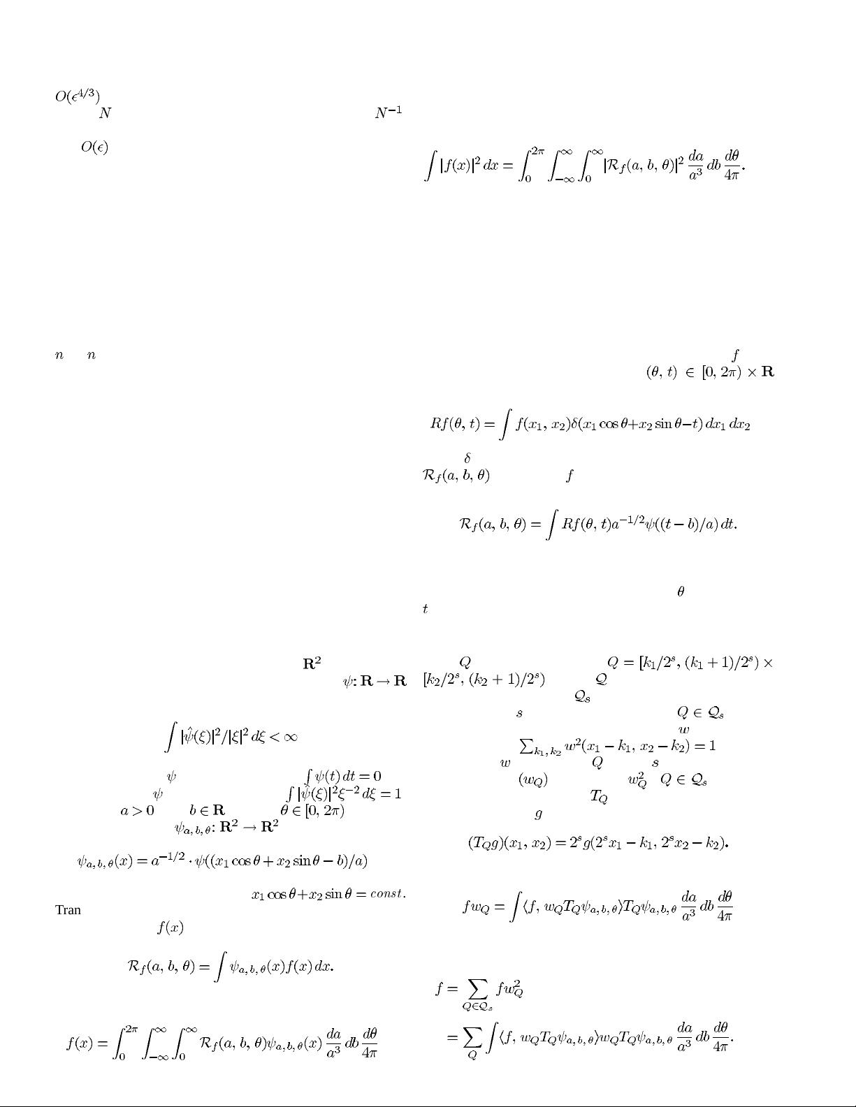
The 2-D continuous ridgelet transform in can be defined

as follows [2]. We pick a smooth univariate function

with sufficient decay and satisfying the admissibility condition

(1)

which holds if, say,

has a vanishing mean .We

will suppose that

is normalized so that .

For each

, each and each , we define

the bivariate ridgelet

(2)

this function is constant along lines

const

Transverse to these ridges it is a wavelet. Given an integrable

bivariate function

, we define its ridgelet coefficients by

We have the exact reconstruction formula

(3)

valid a.e. for functions which are both integrable and square in-

tegrable. Furthermore, this formula is stable as one has a Par-

seval relation

(4)

Hence, much like the wavelet or Fourier transforms, the identity

(3) expresses the fact that one can represent any arbitrary func-

tion as a continuous superposition of ridgelets. Discrete analogs

of (3) and (4) exist; see [2] or [17] for a slightly different ap-

proach.

A. Radon Transform

A basic tool for calculating ridgelet coefficients is to view

ridgelet analysis as a form of wavelet analysis in the Radon do-

main. We recall that the Radon transform of an object

is the

collection of line integrals indexed by

given by

(5)

where

is the Dirac distribution. The ridgelet coefficients

of an object are given by analysis of the Radon

transform via

Hence, the ridgelet transform is precisely the application of a

one-dimensional (1-D) wavelet transform to the slices of the

Radon transform where the angular variable

is constant and

is varying.

B. Ridgelet Pyramids

Let

denote a dyadic square

and let be the collection of all such

dyadic squares. We write

for the collection of all dyadic

squares of scale

. Associated to the squares we con-

struct a partition of energy as follows. With

a nice smooth

window obeying

, we dilate

and transport

to all squares at scale , producing a collec-

tion of windows

such that the s, , make up a

partition of unity. We also let

denote the transport operator

acting on functions

via

With these notations, it is not hard to see that

and, therefore, summing the above equality across squares at a

given scale gives

(6)

剩余14页未读，继续阅读

allew

粉丝: 1
资源: 4

图像去噪：Curvelet变换的应用与实现

曲波变换(Curvelet)融合算法工具箱

第三代小波变换（curvelet）

Transform based image denoising A review.pdf

curvelet--去噪.rar_Curvelet变换_curvelet denoising_去噪_曲波_曲波去噪

Spatial-temporal method for image denoising based on BLS-GSM in curvelet transformation

Multifocus color image fusion based on quaternion curvelet transform

USFFT.rar_curvelet transform_transform

mecv.rar_curvelet_curvelet matlab_curvelet transform_curvelet 变换

CurveLab-2.1.rar_curvelet_curvelet transform

demo.rar_curvelet fusion_curvelet matlab_curvelet transform_fusi

最新资源