noiseless functions get perfect mutual information scores
[21]. Furthermore, the MIC value can be defined as
൫ܦ
௫ǡ௬
൯ൌ
௫௬ழሺሻ
ሼܯሺܦ
௫ǡ௬
ሻሽ
(7)
where ܤ
ሺ
݊
ሻ
is the upper bound of the grid size. In this paper,
we follow [21] to set ܤ
ሺ
݊
ሻ
ൌ݊
Ǥ
as the default value. In
the context of defect prediction, given the class label ܻ, we
calculate the MIC value for each feature ܺ. We rank all orig-
inal features according to their MIC values and select a sub-
set of these features. This will be further explained in Section
III-B.
C. Hierarchical Agglomerative Clustering
We employ a Hierarchical Agglomerative Clustering
(HAC) algorithm to divide features into groups and thus to
reduce redundant features. In Section III-C, we will later
show how to group features via HAC based on the feature
values across software modules. Note that our goal is to
group features rather than modules and features are charac-
terized via their numeric values in software modules.
The clustering process of HAC is described below. First,
the algorithm treats each feature as a cluster and initializes
the distance of every two clusters. Then HAC merges the
nearest two clusters into a new cluster and calculates the
distance between the new cluster and other clusters. The
merging process repeats until a pre-defined criteria reaches
or all features belong to one group [33], [34]. HAC can form
a feature dendrogram of the resulting cluster hierarchy,
which serves as a valuable tool in visualization [35].
The distance between two features can be defined by the
similarity of these features, such as the cosine similarity and
the Pearson correlation coefficient. According to different
distance definitions, there are several kinds of commonly
used linkage methods for calculating the distance between
clusters, such as the single linkage method, the complete
linkage method, and the average linkage method. More de-
tailed description can be found in [36].
In this paper, we determine the final number of clusters
according to a statistic, called inconsistency coefficient dur-
ing clustering (in Section III-D). Based on this statistic, our
method avoids pointing out a specific number of clusters,
which was manually decided in existing work [29], [30].
III. O
UR
P
ROPOSED
A
PPROACH
,
MICHAC
In this section, we first introduce the framework of our
proposed method; then we present the detailed steps in the
stages of feature ranking and feature clustering; finally, we
illustrate how to determine the number of clusters in the
stage of feature clustering.
A. Overview
We propose MICHAC, short for defect prediction via
Maximal Information Coefficient (MIC) with Hierarchical
Agglomerative Clustering (HAC). In MICHAC, we provide
a novel feature selection framework, which combines feature
ranking with feature clustering for defect prediction.
MICHAC selects an optimized subset of module features.
With the support of MICHAC, existing defect prediction
methods, such as Naïve Bayes, can benefit from a high-
quality training dataset that replaces the original one.
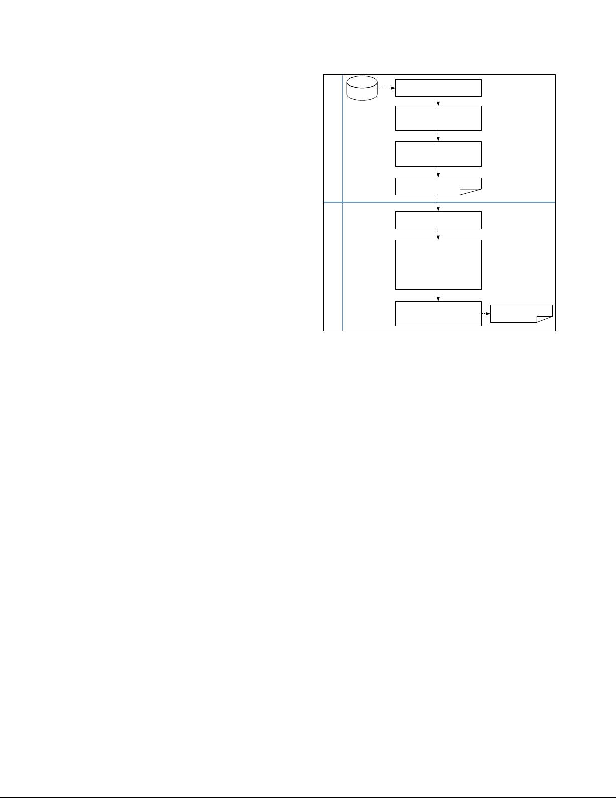
Fig1 illustrates the overall structure of MICHAC. This
structure consists of two major stages: feature ranking and
feature clustering. In the stage of feature ranking, we meas-
ure the relevance of features with respect to the class label
via a new feature ranking technique based on MIC (in Sec-
tion II-B); this stage filters out module features that have a
low correlation with the class label. In the stage of feature
clustering, we cluster features into groups based on HAC (in
Section II-C); this stage eliminates redundant features via
selecting one feature per cluster. As a result, we construct an
optimized subset of module features, which is used to replace
the original feature set in defect prediction.
B. Feature Ranking Stage Based on MIC
In the stage of feature ranking, we mainly conduct the
relevance analysis between each feature with respect to the
class label. That is, features that can distinguish whether a
module is defect-prone or not are selected for the next stage
(in Section III-C). We rank features independently, without
considering any learning algorithm.
The input of feature ranking is a set of defect data,
which can be used to build a predictive model in defect pre-
diction. As shown in Fig. 1, feature ranking consists of three
major steps. In Step n, we preprocess defect data, such as
removing features with only one value and non-numeric
features. In addition, we convert the class label of modules
into binary label. Specifically, we label modules with one or
more defects as 1, otherwise as 0. In Step o, we calculate
the MIC values between each feature ݔ and the class label ݕ
based on Equation 7 in Section II-B. In Step p, we sort all
features based on their MIC values in descending order and
Figure 1. Overview of our proposed approach, MICHAC.
oCompute MIC value for
each feature
pRank features and select
the top p features
qCluster features
rCalculate the increment of
inconsistency coefficient
and determine the cluster
number based on the
maximum increment
sSelect one feature from
each cluster
Feature Ranking
Feature Clustering
Initial feature subset
Raw data
Based on MIC
nPreprocess
Final feature subset
372


