gOMP算法:压缩感知中的高效信号重构
需积分: 9 200 浏览量
更新于2024-07-18
收藏 447KB PDF 举报
广义 Orthogonal Matching Pursuit (gOMP) 是一种在压缩感知领域中备受关注的贪婪算法,它是在传统 Orthogonal Matching Pursuit (OMP) 算法基础上发展起来的一种扩展。OMP 是一种用于从压缩测量数据中重构稀疏信号的有效方法,通过逐次选择与当前残差最匹配的原子来逼近原信号。然而,gOMP 的核心创新在于每次迭代不仅选择一个,而是同时识别多个(N个)"正确"的索引,从而显著减少了所需的迭代次数。
gOMP 的提出旨在提高重构效率,尤其是在处理高维、多稀疏度信号时。相比于原始的 OMP,其性能优势体现在能够使用更少的迭代次数达到同样的重建精度。该算法的关键理论支撑是 Restricted Isometry Property (RIP),即 sensing matrix 必须满足 δ_{NK} < √(N/√(K+3√N)) 条件,这意味着即使信号具有多个非零元素(K>1),gOMP 也能保证完美重建。
实验结果表明,gOMP 在实际应用中的恢复性能非常出色,能够与著名的 l1-minimization 技术相媲美,而且在处理速度上具有明显的优势。由于其快速的计算速度和竞争力的计算复杂度,gOMP 成为了处理大规模稀疏数据的有效工具,特别适合实时应用或者对时间敏感的场景。此外,gOMP 的设计灵活,易于实现,使得它在实际工程中得到了广泛应用,如无线通信、信号处理和机器学习等领域。gOMP 算法的出现,为压缩感知问题的解决提供了一个高效且高效的解决方案,对于推动相关技术的发展具有重要意义。
3
It is worth mentioning that the residual r
k
of the gOMP is
orthogonal to the columns of Φ
Λ
k since
Φ
Λ
k , r
k
=
Φ
Λ
k , P
⊥
Λ
k
y
(4)
= Φ
′
Λ
k
P
⊥
Λ
k
y (5)
= Φ
′
Λ
k
P
⊥
Λ
k
′
y (6)
=
P
⊥
Λ
k
Φ
Λ
k
′
y = 0 (7)
where (6) follows from the symmetry of P
⊥
Λ
k
(P
⊥
Λ
k
=
P
⊥
Λ
k
′
)
and (7) is due to
P
⊥
Λ
k
Φ
Λ
k = (I − P
Λ
k ) Φ
Λ
k = Φ
Λ
k −Φ
Λ
k Φ
†
Λ
k
Φ
Λ
k = 0.
Here we note that this property is satisfied when Φ
Λ
k has
full column rank, which is true if k ≤ m/N in the gOMP
operation. It is clear from this observation that indices in
Λ
k
cannot be re-selected in the succeeding iterations and the
cardinality of Λ
k
becomes simply kN. When the iteration loop
of the gOMP is finished, therefore, it is possible that the final
support set Λ
s
contains indices not in T . Note that, even in
this situation, the final result is unaffected and the original
signal is recovered because
ˆ
x
Λ
s
= Φ
†
Λ
s
y (8)
= (Φ
′
Λ
s
Φ
Λ
s
)
−1
Φ
′
Λ
s
Φ
T
x
T
(9)
= (Φ
′
Λ
s
Φ
Λ
s
)
−1
Φ
′
Λ
s
(Φ
Λ
s
x
Λ
s
)
−(Φ
′
Λ
s
Φ
Λ
s
)
−1
Φ
′
Λ
s
Φ
Λ
s
−T
x
Λ
s
−T
(10)
= x
Λ
s
, (11)
where (10) follows from the fact that x
Λ
s
−T
= 0. From
this observation, we deduce that as long as at least one
correct index is found in each iteration of the gOMP, we can
ensure that the original signal is perfectly recovered within K
iterations. In practice, however, the number of correct indices
being selected is usually more than one so that the required
number of iterations is much smaller than K.
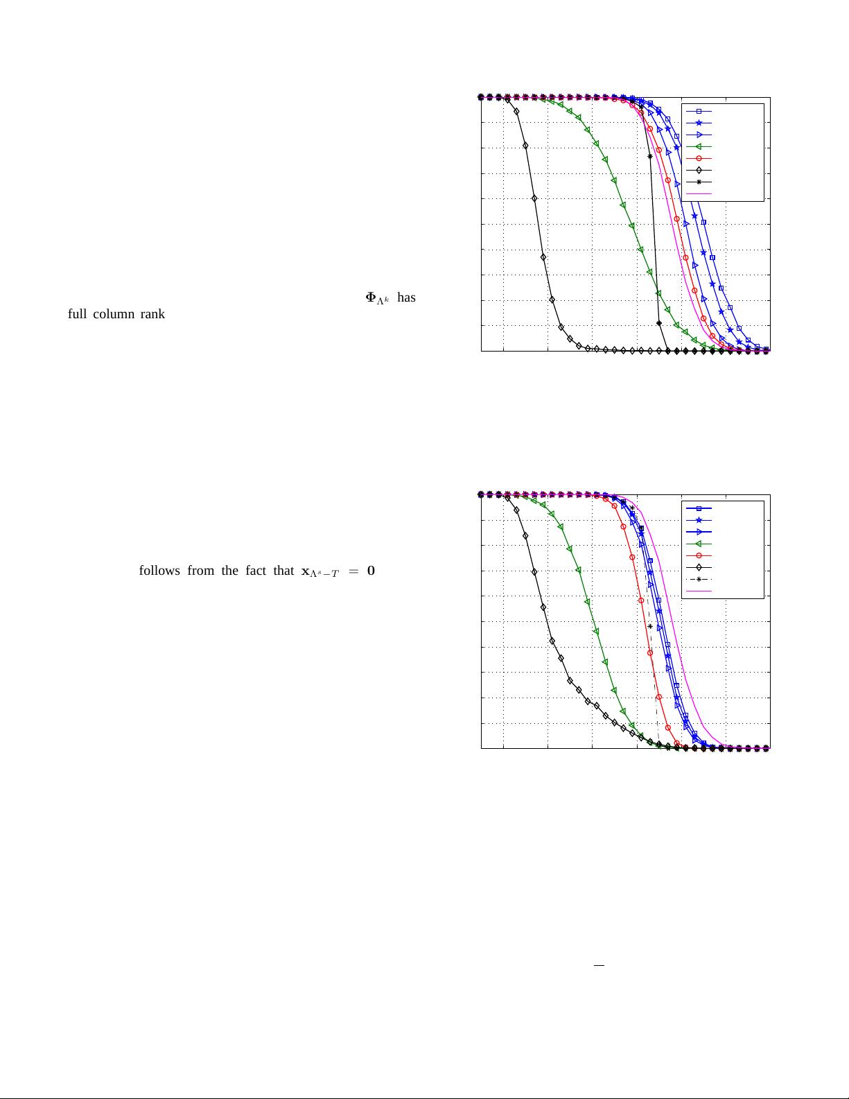
In order to observe the empirical performance of the gOMP
algorithm, we performed computer simulations. In our ex-
periment, we use the testing strategy in [16], [22] which
measures the effectiveness of recovery algorithms by checking
the empirical frequency of exact reconstruction in the noiseless
environment. By comparing the maximal sparsity level of
the underlying sparse signals at which the perfect recovery
is ensured (this point is often called critical sparsity [16]),
accuracy of the reconstruction algorithms can be compared
empirically. In our simulation, the following algorithms are
considered.
1) LP technique for solving ℓ
1
-minimization problem
(http://cvxr.com/cvx/).
2) OMP algorithm.
3) gOMP algorithm.
4) StOMP with false alarm control (FAC) based threshold-
ing (http://sparselab.stanford.edu/).
1
5) ROMP algorithm
(http://www.cmc.edu/pages/faculty/DNeedell).
1
Since FAC scheme outperforms false discovery control (FDC) scheme, we
exclusively use FAC scheme in our simulation.
10 20 30 40 50 60 70
0
0.1
0.2
0.3
0.4
0.5
0.6
0.7
0.8
0.9
1
Sparsity
Frequency of Exact Reconstruction
gOMP (N=3)
gOMP (N=6)
gOMP (N=9)
OMP
StOMP
ROMP
CoSaMP
LP
Fig. 1. Reconstruction performance for K-sparse Gaussian signal vector as
a function of sparsity K.
10 20 30 40 50 60 70
0
0.1
0.2
0.3
0.4
0.5
0.6
0.7
0.8
0.9
1
Sparsity
Frequency of Exact Reconstruction
gOMP (N=3)
gOMP (N=6)
gOMP (N=9)
OMP
StOMP
ROMP
CoSaMP
LP
Fig. 2. Reconstruction performance for K-sparse PAM signal vector as a
function of sparsity K.
6) CoSaMP algorithm
(http://www.cmc.edu/pages/faculty/DNeedell).
In each trial, we construct m ×n (m = 128 and n = 256)
sensing matrix Φ with entries drawn independently from
Gaussian distribution N(0,
1
m
). In addition, we generate a
K-sparse vector x whose support is chosen at random. We
consider two types of sparse signals; Gaussian signals and
pulse amplitude modulation (PAM) signals. Each nonzero
element of Gaussian signals is drawn from standard Gaussian
剩余14页未读,继续阅读
2018-09-12 上传
2021-05-27 上传
2020-06-27 上传
2021-05-29 上传
2021-09-29 上传
2022-09-23 上传

tongzs2017
- 粉丝: 2
- 资源: 3
 我的内容管理
展开
我的内容管理
展开


最新资源
- 高清艺术文字图标资源,PNG和ICO格式免费下载
- mui框架HTML5应用界面组件使用示例教程
- Vue.js开发利器:chrome-vue-devtools插件解析
- 掌握ElectronBrowserJS:打造跨平台电子应用
- 前端导师教程:构建与部署社交证明页面
- Java多线程与线程安全在断点续传中的实现
- 免Root一键卸载安卓预装应用教程
- 易语言实现高级表格滚动条完美控制技巧
- 超声波测距尺的源码实现
- 数据可视化与交互:构建易用的数据界面
- 实现Discourse外聘回复自动标记的简易插件
- 链表的头插法与尾插法实现及长度计算
- Playwright与Typescript及Mocha集成:自动化UI测试实践指南
- 128x128像素线性工具图标下载集合
- 易语言安装包程序增强版:智能导入与重复库过滤
- 利用AJAX与Spotify API在Google地图中探索世界音乐排行榜
