光束法平差：现代计算机视觉重建关键理论综述

5星 · 超过95%的资源 190 浏览量更新于2024-07-18 1 收藏 624KB PDF 举报

光束法平差(Bundle Adjustment)是一种现代摄影测量技术的核心组成部分，它在计算机视觉领域中扮演着关键角色，旨在通过优化结构和观测参数来提升图像重建的质量。这篇英文文献由Bill Triggs、Philip McLauchlan、Richard Hartley和Andrew Fitzgibbon四位专家撰写，他们分别来自法国INRIA Rhône-Alpes、英国萨里大学、美国通用电气研究与发展中心以及英国牛津大学。本文的主要目标是对摄影测量中的光束法平差理论和方法进行深入剖析，以供计算机视觉社区的潜在实现者参考。光束法平差的核心问题在于如何通过调整多视图影像中的相机位置、姿态（即结构参数）以及相对几何关系（即观测参数），使得整个视觉重建达到全局最优。这涉及到以下几个关键主题： 1. 成本函数与鲁棒性：选择合适的成本函数至关重要，因为它决定了优化过程对误差的敏感程度。一个有效的成本函数应该既能反映数据的精确性，又能处理异常值，提高系统的鲁棒性。 2. 数值优化：包括使用稀疏牛顿方法，这是一种高效的求解策略，能在大规模数据集上进行计算。此外，文中还讨论了线性收敛近似算法，它们能够在一定程度上加速优化过程，减少迭代次数。 3. 度量不变性（Gauge Invariance）：光束法平差必须处理不同度量系统下的几何一致性，确保结果不受相机坐标系或基准变换的影响。这要求算法具备一定的内在稳定性，使得结果在不同的度量框架下保持一致。 4. 质量控制：为了保证优化过程的稳定性和可靠性，文中讨论了如何监控和评估优化结果的质量，如残差分析、自检验机制等，这些对于防止陷入局部最优解具有重要意义。这篇文章详尽地介绍了光束法平差的各个方面，不仅涵盖理论基础，还包括实际应用中的技巧和策略。对于从事摄影测量、三维重建或者计算机视觉领域的研究者和工程师来说，理解和掌握这些内容将有助于他们在实践中提升精度和效率。

310 B. Triggs et al.

outliers are entirely ignored. The dispersion matrix W

−1

determines the spatial spread of z

and up to scale its covariance (if this is ﬁnite). The radial form is preserved under arbitrary

afﬁne transformations of z

, so within a group, all of the observations are on an equal

footing in the same sense as in least squares. However, non-Gaussian radial distributions

are almost never separable: the observations in z

can neither be split into independent

subgroups, nor combined into larger groups, without destroying the radial form. Radial

cost models do not have the remarkable isotropy of non-robust SSE, but this is exactly

what we wanted, as it ensures that all observations in a group will be either left alone, or

down-weighted together.

As an example of this, for image features polluted with occasional large outliers caused

by correspondence errors, we might model the error distribution as a Gaussian central peak

plus a uniform background of outliers. This would give negative log likelihood contribu-

tions of the form f(x)=−log



exp(−

)+



instead of the non-robust weighted

SSE model f(x)=

, where χ

= x



x

is the squared weighted residual

error (which is a χ

variable for a correct model and Gaussian error distribution), and 

parametrizes the frequency of outliers.

-10 -5 0 5 10

Gaussian -log likelihood

Robustified -log likelihood

3.4 Intensity-Based Methods

The above models apply not only to geometric image features, but also to intensity-based

matching of image patches. In this case, the observables are image gray-scales or colors

I rather than feature coordinates u, and the error model is based on intensity residuals.

To get from a point projection model u = u(x) to an intensity based one, we simply

compose with the assumed local intensity model I = I(u) (e.g. obtained from an image

template or another image that we are matching against), premultiply point Jacobians by

point-to-intensity Jacobians

, etc. The full range of intensitymodelscanbe implemented

within this framework: pure translation, afﬁne, quadratic or homographic patch deforma-

tion models, 3D model based intensity predictions, coupled afﬁne or spline patches for

surface coverage, etc., [1, 52, 55,9,110, 94, 53, 97, 76,104,102]. The structure of intensity

based bundle problems is very similar to that of feature based ones, so all of the techniques

studied below can be applied.

We will not go into more detail on intensity matching, except to note that it is the

real basis of feature based methods. Feature detectors are optimized for detection not

localization. To localize a detected feature accurately we need to match (some function of)

Bundle Adjustment — A Modern Synthesis 311

the image intensities in its region against either an idealized template or another image of

the feature, using an appropriate geometric deformation model, etc. For example, suppose

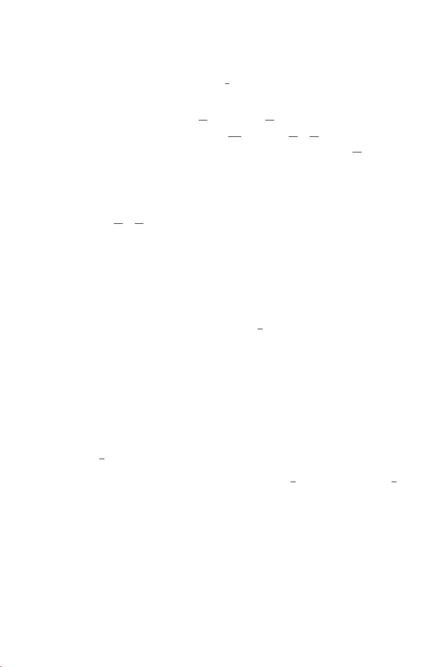
that the intensity matching model is f(u)=



ρ(δI(u)

) where the integration is

over some image patch, δI is the current intensity prediction error, u parametrizes the local

geometry (patch translation & warping), and ρ(·) is some intensity error robustiﬁer. Then

the cost gradient in terms of u is g







δI



. Similarly, the cost Hessian in

u in a Gauss-Newton approximation is H

≈





(

)



. In a feature based

model, we express u = u(x) as a function of the bundle parameters, so if J

we have

a corresponding cost gradient and Hessian contribution g



= g



and H

= J



In other words, the intensity matching model is locally equivalent to a quadratic feature

matching one on the ‘features’ u(x), with effective weight (inverse covariance) matrix

= H

. All image feature error models in vision are ultimately based on such an

underlying intensity matching model. As feature covariances are a function of intensity

gradients





(

)



, they can be both highly variable between features (depending

on how much local gradient there is), and highly anisotropic (depending on howdirectional

the gradients are). E.g., for points along a 1D intensity edge, the uncertainty is large in the

along edge direction and small in the across edge one.

3.5 Implicit Models

Sometimes observations are most naturally expressed in terms of an implicit observation-

constraining model h(x, z)=0, rather than an explicit observation-predicting one z =

z(x). (The associated image error still has the form f(z

− z)). For example, if the model

is a 3D curve and we observe points on it (the noisy images of 3D points that may lie

anywhere along the 3D curve), we can predict the whole image curve, but not the exact

position of each observation along it. We only have the constraint that the noiseless image

of the observed point would lie on the noiseless image of the curve, if we knew these. There

are basically two ways to handle implicit models: nuisance parameters and reduction.

Nuisance parameters: In this approach, the model is made explicit by adding additional

‘nuisance’ parameters representing something equivalent to model-consistent estimates

of the unknown noise free observations, i.e.toz with h(x, z)=0. The most direct way

to do this is to include the entire parameter vector z as nuisance parameters, so that we

have to solve a constrained optimization problem on the extended parameter space (x, z),

minimizing f(z

− z) over (x, z) subject to h(x, z)=0. This is a sparse constrained

problem, which can be solved efﬁciently using sparse matrix techniques (§6.3). In fact,

for image observations, the subproblems in z (optimizing f(z

− z) over z for ﬁxed z

and x) are small and for typical f rather simple. So in spite of the extra parameters z,

optimizing this model is not signiﬁcantly more expensive than optimizing an explicit one

z = z(x) [14, 13, 105, 106]. For example, when estimating matching constraints between

image pairs or triplets [60, 62], instead of using an explicit 3D representation, pairs or

triplets of corresponding image points can be used as features z

, subject to the epipolar

or trifocal geometry contained in x [105, 106].

However, if a smaller nuisance parameter vector than z can be found, it is wise to use

it. In the case of a curve, it sufﬁces to include just one nuisance parameter per observation,

saying where along the curve the corresponding noise free observation is predicted to

lie. This model exactly satisﬁes the constraints, so it converts the implicit model to an

unconstrained explicit one z = z(x, λ), where λ are the along-curve nuisance parameters.

312 B. Triggs et al.

The advantage of the nuisance parameter approach is that it gives the exact optimal

parameter estimate for x, and jointly, optimal x-consistent estimates for the noise free

observations z.

Reduction: Alternatively, we can regard h(x, z

) rather than z as the observation vector,

and hence ﬁt the parameters to the explicit log likelihood model for h(x, z

). To do this,

we must transfer the underlying error model / distribution f(z) on z

to one f(h) on

h(x, z

). In principle, this should be done by marginalization: the density for h is given

by integrating that for z over all z giving the same h. Within the point estimation

framework, itcan be approximated byreplacingthe integrationwithmaximization. Neither

calculation is easy in general, but in the asymptotic limit where ﬁrst order Taylor expansion

h(x, z

)=h(x, z + z) ≈ 0 +

z is valid, the distribution of h is a marginalization or

maximization of that of z over afﬁne subspaces. This can be evaluated in closed form for

some robust distributions. Also, standard covariance propagation gives (more precisely,

this applies to the h and z dispersions):

h(x, z

)≈0 , h(x, z) h(x, z)



≈

z z







−1



(4)

where W

−1

is the covariance of z. So at least for an outlier-free Gaussian model, the

reduced distribution remains Gaussian (albeit with x-dependent covariance).

4 Basic Numerical Optimization

Having chosen a suitable model quality metric, we must optimize it. This section gives a

very rapid sketch of the basic local optimization methods for differentiable functions. See

[29, 93,42] for more details. We need to minimize a cost function f(x) over parameters x,

starting from some given initial estimate x of the minimum, presumably supplied by some

approximatevisualreconstruction methodorprior knowledgeofthe approximatesituation.

As in §2.2, the parameter space may be nonlinear, but we assume that local displacements

can be parametrized by a local coordinate system / vector of free parameters δx.Wetry

to ﬁnd a displacement x → x + δx that locally minimizes or at least reduces the cost

function. Real cost functions are too complicated to minimize in closed form, so instead

we minimize an approximate local model for the function, e.g. based on Taylor expansion

or some other approximation at the current point x. Although this does not usually give the

exact minimum, with luck it will improve on the initial parameter estimate and allow us to

iterate to convergence. The art of reliable optimization is largely in the details that make

this happen even without luck: which local model, how to minimize it, how to ensure that

the estimate is improved, and how to decide when convergence has occurred. If you not

are interested in such subjects, use a professionally designed package (§C.2): details are

important here.

4.1 Second Order Methods

The reference for all local models is the quadratic Taylor series one:

f(x + δx) ≈ f(x)+g



δx +

δx



H δxg≡

(x) H ≡

(x)

quadratic local model gradient vector Hessian matrix

(5)

剩余74页未读，继续阅读

tianjianbowu

粉丝: 2
资源: 8

光束法平差：现代计算机视觉重建关键理论综述

光束法区域网平差vc代码

影像匹配，光束法区域网平差

光束法平差模型

sba-1.6_光束_光束法平差_光束法_sba—1.6_

近景摄影测量光束法平差

光束法平差模型的具体推导

sba一个光束法平差解释

旋转矩阵四元素法和光束法平差模型.doc

基于点松弛法的自检校光束法平差快速计算

消元法在光束法平差中的应用[收集].pdf

最新资源