NSGA2约束处理：优化化工批量装置设计中的非线性策略

2星需积分: 46 53 浏览量更新于2024-07-21 10 收藏 1.24MB PDF 举报

"遗传算法在优化过程中面临着如何有效地处理约束条件的问题，特别是在解决大规模和复杂问题时，如化工过程中的最优批量工厂设计。本文主要探讨了NSGA2（非支配排序遗传算法第二版）在面对非线性约束时的处理策略，这在化学工程和加工领域是一个重要的研究课题。 NSGA2是一种多目标优化算法，特别适合处理包含多个目标函数和约束条件的混合整数非线性规划（MINLP）问题。然而，原始的遗传算法设计可能并不完美地适应所有类型的约束，例如时间限制、物料平衡、反应速率限制等。这些问题如果不能直接融入变量编码或通过调整遗传操作来考虑，就可能导致算法性能下降，甚至可能导致搜索陷入局部最优。本文作者A.Ponsich、C.Azzaro-Pantel、S.Domenech和L.Pibouleau在Toulouse的化学工程实验室进行了一项研究，他们选择了一个中等规模的工厂设计案例来测试几种不同的约束处理技术。这些技术可能包括：解空间划分、惩罚函数、松弛约束、二进制编码与连续解之间的转换方法，以及动态调整适应度函数等。研究的目的是为了找出哪种约束处理方法在实际应用中能提供最有效的解决方案，同时保持算法的稳健性和收敛性。通过对比不同策略的效果，研究人员可以为其他工程师提供关于如何在遗传算法中更有效地处理约束条件的指导，从而提升整个优化过程的效率和结果的质量。总结来说，这篇论文的核心内容是针对NSGA2在化工过程优化中的约束处理技巧，其目标是通过实证分析找到最佳实践，以应对复杂的约束问题，并为该领域的实践者提供有价值的参考。"

422 A. Ponsich et al. / Chemical Engineering and Processing 47 (2008) 420–434

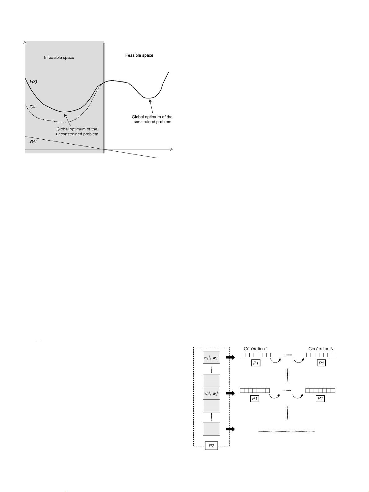
Fig. 1. Too weak penalty factor.

According to these principles, a great variety of penalisa-

tion methods were implemented, some of them are recalled in

[14]. The simplest is the static penalty: a numerical value, that

will not vary during the whole search, is allocated to each fac-

tor R

. Obviously, the drawback is that as many parameters as

existing constraints have to be tuned without any known method-

ology. Normalizing the constraints enables however to reduce

the number of parameters to be chosen from m to 1.

A modiﬁed static penalty technique is proposed in [15],in

which violation levels are set for each constraint. So considering

l levels in a problem with m constraints, it was shown that the

method needs the tuning of m(2l + 1) parameters (see [14] for

details).

Another proposal is a dynamic penalty strategy, for which R

is written as (C × t)

where t is the generation number. Here,

two parameters must be tuned, i.e. C and a. Common values are

0.5 and 2, respectively. Thus, this method enables to increase

the pressure on infeasible solutions along the search. A similar

effect can be obtained with a method presenting an analogy with

Simulated Annealing:

(3)

where τ is a decreasing temperature. It is necessary to determine

initial and ﬁnal temperatures, τ

and τ

, as well as a cooling

scheme for τ. This technique has two special features. First, it

involves a difference between linear and non-linear constraints.

Feasibility as regard with the former is maintained by speciﬁc

operators, so that only the latter has to be included in the anneal-

ing penalty term. In addition, the initial population is composed

of clones of a same feasible individual that respects linear con-

straints [14].

Different approaches, called adaptive penalties, are based on

learning from the population behaviour in the previous gener-

ations. In [16], the penalty factor decreases (resp. increases) if

the best individual was always feasible (resp. infeasible) during

the k last generations. For undeterminated cases, the factor value

is kept unchanged. This methodology imposes the tuning of the

initial value for the penalty factor and of the number of learning

generations k.

New techniques now rest on self-adaptive penalty

approaches, which also learn from the current run, without any

parameter tuning. In [13], the constraints and the objective func-

tion are ﬁrst normalized. Then, the method consists in computing

the penalty factor for constraint j at generation q as the product

of the factor at generation q − 1 with a coefﬁcient depending on

the ratio of individuals violating constraint j at generation q.If

this ratio is fewer to 50%, then the coefﬁcient is inferior to 1

in order to favour individuals located in the infeasible side of

the boundary. On the contrary, if the feasible individuals num-

ber is weak, the value increases up to 1 to have the population

heading for the inside part of the feasible region. This oper-

ating mode enables to concentrate the search on the boundary

built by each constraint, i.e. where the global optimum is likely

to be located. The initial value is the ratio of the interquartile

range of the objective function by the interquartile range of the

considered constraint at ﬁrst generation, which implicitly car-

ries out normalization. No parameter is thus necessary in this

method.

Another kind of self-adaptive penalty is proposed by Coello

Colleo [17], but this one is based on the principle of co-evolution.

In addition to the classical population P1 coding the tackled

problem, the method considers a population P2 representing two

penalty coefﬁcients that enable to evaluate population P1 (w

for

the amount of violation of all constraints and w

for the number

of violated constraints). Thus, each individual of P1 is evaluated

as many times as there are individuals in P2. Then, P1 evolves

during a ﬁxed number of generations and each individual of P2,

i.e. each set of two penalty factors, is evaluated. This mechanism

is depicted in Fig. 2. Basically, the evaluation is calculated as the

average of all objective functions of P1 evaluated by each indi-

vidual of P2. Then P2 evolves like in any GA process, given that

one generation for P2 is equivalent to a complete evolution of P1.

The evident drawback is the huge number of objective function

evaluations, making this method computationally expensive. In

addition, co-evolution involves the introduction and tuning of a

new GAs parameters set: population size, maximum generation

number, etc.

Fig. 2. Self-adaptive penalty by co-evolution [17].

剩余14页未读，继续阅读

robot_junior

粉丝: 5
资源: 7

NSGA2约束处理：优化化工批量装置设计中的非线性策略

惩罚函数法在遗传算法处理约束问题中的应用

带有约束条件的遗传算法程序

解整数规划的0-1遗传算法

数学建模-机构设计的遗传算法约束条件处理.zip

遗传算法约束条件matlab

matlab遗传算法约束条件

myDearGA.rar_dear.ga_planmua_有约束条件_遗传算法约束

基于遗传算法多约束条件下的供应商选择研究

遗传算法约束处理新方法：可行解与不可行解混合交叉

遗传算法求解约束条件的应用及标注解析

最新资源