出租车司机乘客推荐系统：基于GPS轨迹的高效匹配策略

需积分: 10 82 浏览量更新于2024-09-10 收藏 2.48MB PDF 举报

本文主要探讨的是"A Recommender System for Finding Passengers and Vacant Taxis"，一种针对出租车司机和乘客需求的推荐系统。该系统利用出租车GPS轨迹数据，深入分析乘客的移动模式和司机的接客/送客行为，旨在提高服务效率并优化收益。首先，该推荐系统为出租车司机提供一系列可能的目的地，这些地方更有可能快速接到乘客，尤其是在行程中或者目的地附近。系统通过学习大量出租车的GPS轨迹数据，推算出不同地点对于司机来说接客概率较高的规律，从而生成个性化的建议，帮助司机规划更有效的路线，增加下一次出行的盈利机会。其次，对于寻找空车的乘客，系统同样提供推荐功能。它会推荐在步行距离内、容易找到空车的位置，基于司机的实际需求时间点，结合学习到的概率模型，预测在特定时刻和地点推荐候选位置对司机的潜在利润。这样做的目的是为了减少乘客等待时间，提高乘客体验，并在供需匹配中实现双赢。在实施上，作者团队利用了超过12,000辆出租车的历史轨迹数据进行模型训练，确保推荐的准确性。这种方法不仅依赖于大数据的处理能力，还涉及到机器学习算法，如概率模型，来处理复杂的交通动态和乘客行为预测。这个推荐系统是一项结合了地理位置、移动行为分析和收益预测的创新技术，它通过智能化的方式优化了出租车行业的运营效率和服务质量，提升了乘客和司机的满意度。这种应用对于提升城市交通系统的整体效能，降低拥堵，以及推动共享经济的发展都具有重要意义。

0 1 2 3 4 5 6 7

fare distance/unit time (m/s)

cruising distance/unit time (m/s)

density−→

r = 0. 0874

Fig. 2. Density scatter of cruising distance/unit time w.r.t.

proﬁt

Trajectories

Parking Detection

Parking places

Segmentation

Trips

Map-MatchingStatistic learning

Knowledge of

road segments

Offline Mining

Knowledge of

parking places

Taxi Recommender Passenger Recommender

Online Recommendation

Fig. 3. System Overview

outperforms other approaches for low-sampling-rate GPS

trajectories. Later, we utilize the detected parking places

and the mapped trajectories to learn the time-dependent

statistical results based on a probabilistic model (Section 4).

To tackle the data sparseness problem, we devise a road

segment clustering method and perform statistical learning on

each road segment cluster instead of a single road segment

(Section 5). The above processes are performed ofﬂine and

will be repeated only when the trajectory data is updated

(e.g., once a month). Based on this model, we perform

recommendations to taxi drivers and passengers, given their

locations and current times (Section 6).

3 PARKING PLACES DETECTION

This section details the process for detecting parked status

from a non-occupied trip and accordingly ﬁnding out the

parking places in the urban area of a city based on a collection

of taxi trajectories.

3.1 Candidates Detection

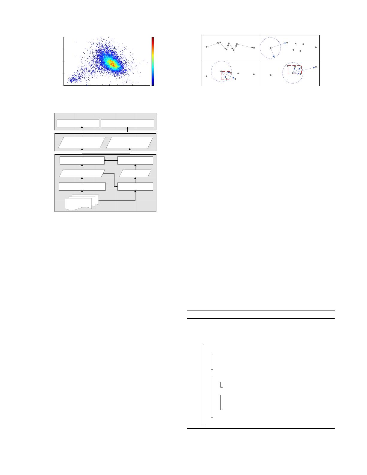
Figure 4 demonstrates the parking candidate detection ap-

proach, given a non-occupied trip p

→ p

→ · · · → p

We ﬁrst keep checking the distance (Great-circle distance)

between the current point and the latter point until the

distance is smaller than a threshold. As depicted in Figure

4 B), since dist(p

, p

) exceeds the distance threshold δ,

we move next, ﬁxing p

as the “pivot” point and ﬁnd that

dist(p

, p

) < δ, dist(p

, p

) < δ while dist(p

, p

) > δ

(A)

(B)

(C)

(D)

Fig. 4. Detection of candidate parking places

(Figure 4 C). If the time interval between p

.t and p

.t is

larger than the time threshold τ , the three points that form

a small cluster represent a possible parking candidate. Next,

we ﬁx p

as the pivot point and keep on the procedure to

check latter points. Finally, as shown in Figure 4 D), we

detect (p

, p

) as a parking candidate because we

cannot expand this group any further, i.e., all the points in this

group have a distance farther than δ to p

. The pseudocode

is provided in Algorithm 1.

3.2 Filtering

Essentially, the candidate detection algorithm ﬁnds out the lo-

cations where the GPS points of a taxi are densely clustered,

with spatial and temporal constraints. However, a parking

candidate could sometimes be generated by taxis stuck in a

trafﬁc jam, or waiting for signals at a trafﬁc light, instead of

a real parking. To reduce such false selections, we design a

supervised model for picking out the true parked status from

the candidate set, using the following features:

• Spatial-Temporal features including 1) Minimum

Bounding Ratio (MBR). As shown in Figure 5(A),B)),

MBR is the area ratio between the bounding box of

the road segment (MBRr) and the bounding box of

the GPS points (MBRc) in the candidate set. 2) Av-

erageDistance. The average distance d

between points

in the candidate set and their nearest road segments, as

Algorithm 1: ParkingCandidateDetection

Input: A road network G, a trajectory J, distance threshold δ, time

threshold τ

Output: A set of parking candidates P = {P }

1 i ← 0, M ← kJk, P ← ∅, P ← ∅;

2 while i < (M − 1) do

3 j ← i + 1; ﬂag ←false;

4 while j < M do

5 dist ←Distance (p

, p

);

6 if dist < δ then j ← j + 1;ﬂag =true;

7 else break;

8 if p

j−1

.t − p

.t > τ and ﬂag =true then

9 foreach point p ∈ J[i, j) and p /∈ P do

10 P .Add(p);/

build a candidate

11 if i = j − 1 then

12 P.Add(MB (P)); P ← ∅;

add the minimum bounding box of P

into P

13 i ← i + 1;

14 return P

剩余13页未读，继续阅读

ljpeng234

粉丝: 0
资源: 1

出租车司机乘客推荐系统：基于GPS轨迹的高效匹配策略

A Group Specific Recommender System

Deep Learning based Recommender System: A Survey and New Perspectives

Deep Learning based Recommender System- A Survey and New Perspectives.pdf

Recommender System

recommender system

A Hybrid Movie Recommender System Based on Neural Networks

《Wide & Deep Learning for Recommender System》翻译1

Building a better recommender system in E-commerce (2003年)

Exploring Social Tagging in a Web 2.0 Recommender System.pdf

LARS__ An Efficient and Scalable Location-Aware Recommender System

最新资源