并发广度优先搜索(iBFS)在GPU上的实现与优化

72 浏览量更新于2024-08-25 收藏 1.17MB PDF 举报

"iBFS - Concurrent Breadth-First Search on GPUs - 2016 (ibfs_tcm18-284417)-计算机科学" 本文介绍了一种名为iBFS（并发广度优先搜索）的算法，该算法针对图形处理单元（GPU）进行了优化，用于高效执行多源节点的并发BFS。传统的BFS是一种关键的图算法，具有广泛的应用，例如在社交网络分析、路由算法和最短路径查找等领域。然而，同时进行多个BFS遍历以提高效率和探索更多可能性的需求催生了并发BFS的研究。作者Hang Liu、H. Howie Huang和Yang Hu来自乔治华盛顿大学的电气与计算机工程系。他们设计并实现了iBFS，这是一种新的方法，能够有效地在GPU上运行并发BFS任务。以下是iBFS的核心特点： 1. **单一GPU内核**：iBFS创新地使用了一个单一的GPU内核来实现并发BFS，使得不同实例间的共享前沿能够被充分利用。这意味着不同BFS遍历可以并行进行，并且能够有效地协调共享数据，从而提高整体性能。 2. **基于出度的GroupBy规则**：iBFS通过基于出度的分组策略选择性地运行BFS实例。这一规则有助于最大化同一组内实例之间的前沿共享，减少了数据冗余和通信开销，进一步提升了性能。 3. **优化的位操作**：iBFS利用GPU上的高度优化的位操作技术，使单个GPU线程能够快速检查和处理大量信息。这提高了处理速度，使得在大规模图数据上执行并发BFS变得更为高效。 iBFS的这些设计不仅减少了GPU资源的浪费，还显著增强了并发性能。在大数据和复杂图形分析的背景下，这种优化对于提高计算效率至关重要。通过并发处理，iBFS能够更有效地应对大规模图结构中的并行任务，同时保持低延迟和高吞吐量。 iBFS是GPU计算领域的一个重要突破，它展示了如何通过创新算法设计和硬件特性利用，将图形算法的性能推向新的高度。对于需要处理大量图数据的领域，如社交网络分析、网络路由、生物信息学和机器学习等，iBFS提供了强大且高效的解决方案。

256

FB FR HW KG0 KG1 KG2 LJ OR PK RD RM TW WK

Frontier sharing percentage (log scale)

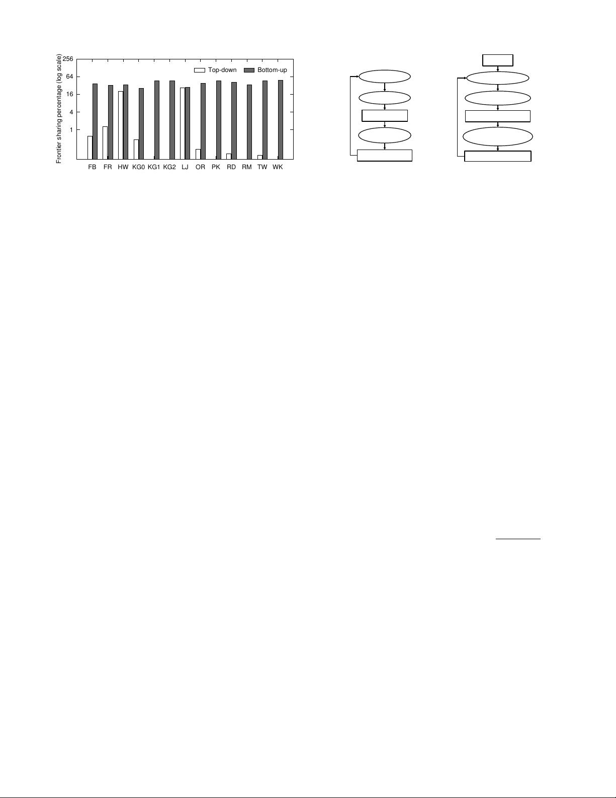
Top-down Bottom-up

Figure 2: Average frontier sharing percentage between two diﬀer-

ent BFS instances.

Among three tasks at each level, inspecting adjacent ver-

tices of the frontiers involves a lot of random memory ac-

cesses (pointer-chasing), accounting for most of the runtime.

This can be observed on four BFS traversals for both top-

down and bottom-up in Figure 1.

Concurrent BFS executes multiple BFS instances from

diﬀerent source vertices. Using the example in Figure 1, four

BFS instances start from vertex 0, 3, 6, and 8, respectively.

A naive implementation of concurrent BFS will run all BFS

instances separately and keep its own private frontier queue

and status array. On a GPU device, each individual subrou-

tine is deﬁned as a Kernel. Therefore, in the aforementioned

example, four kernels will run four BFS instances in parallel

from four source vertices. NVIDIA Kepler provides Hyper-Q

to support concurrent execution of multiple kernels, which

dramatically increases the GPU utilization especially when

a single kernel cannot fully utilize the GPU [34].

Unfortunately, this naive implementation of concurrent

BFS takes approximately the same amount of time as run-

ning these BFS instances sequentially, as we will show later

in Section 8. For example, for all the graphs evaluated

in this paper, sequential and naive implementation of con-

current BFS take average 52 ms and 48 ms, respectively,

with a diﬀerence in traversal rate of 500 million TEPS. The

main reason for such a small beneﬁt is because simply run-

ning multiple BFS instances in parallel would overwhelm the

GPU, especially at the direction-switching level when a BFS

goes from top-down to bottom-up. At that moment each

individual BFS would require a large number of threads for

their workloads. As a result, such a naive implementation

may even underperform a sequential execution of all BFS

instances.

Opportunity of Frontier Sharing: iBFS aims to address

this problem by leveraging the existence of frontiers shared

among diﬀerent BFS instances. Figure 2 presents the av-

erage percentage of shared frontiers per level between two

instances. The graphs used in this paper are presented in

Section 8. Top-down levels have smaller number of shared

frontiers (close to 4% on average) whereas bottom-up levels

have much more as high as 48.6%. This is because bottom-

up traversals often start from a large number of unvisited

vertices (frontiers in this case) and search for their parents.

The proposed GroupBy technique can improve the sharing

for both directions to 10× and 1.7×, respectively.

Potentially, the shared frontiers can yield three beneﬁts in

concurrent BFS: (1). These frontiers need to be enqueued

only once into the frontier queue. (2). The neighbors of

shared frontiers need to be loaded in-core only once during

Status&Array&

Fron-er&Queue&

Expansion&

Inspec-on&

FQ&Genera-on&

Bitwise'Status'Array''

Joint'Fron2er'Queue'

Bitwise'Fron2er''

Iden2ﬁca2on''

Bitwise'Inspec2on''

Joint'Expansion'

GroupBy'

(a) A Single BFS (b) iBFS

Figure 3: The ﬂow charts of (a) BFS, (b) iBFS.

expansion. (3). Memory accesses to the statuses of those

neighbors for diﬀerent BFSes can be coalesced. It is impor-

tant to note that each BFS still has to inspect the statuses

independently, because not all BFSes will have the same sta-

tuses for their neighbors. In other words, shared frontiers

do not reduce the overall workload. Nevertheless, this work

proposes that shared frontiers can be utilized to oﬀer faster

data access and saving in memory usage, both of which are

critical on GPUs. This is achieved through a combination

of bitwise, joint traversals and GroupBy rules that guide the

selection of groups of BFSes for parallel execution.

3. iBFS OVERVIEW

In a nutshell, iBFS as shown in Figure 3, consists of three

unique techniques, namely, joint traversal, GroupBy, and

bitwise optimization, which will be discussed in Section 4,

5, and 6, respectively.

Ideally the best performance for iBFS would be achieved

by running all i BFS instances together without GroupBy.

Unfortunately, ever-growing graph sizes, combined with lim-

ited GPU hardware resources, puts a cap on the number of

concurrent BFS instances. In particular, we have found that

GPU global memory is the dominant factor, e.g., 12GB on

K40 GPUs compared to many TB-scale graphs.

Let M be GPU memory size and N the maximum number

of concurrent BFS instances in one group (i.e., the group

size). If the whole graph requires S storage, a single BFS

instance needs |SA| to store its data structures (e.g., the

status array for all the vertices), and for a joint traversal

each group requires at least |JF Q| for joint data structures

(e.g., the joint frontier queue), then N 6

M−S−|JF Q|

|SA|

. In

most cases N satisﬁes 1 < N  i 6 |V |. In this paper, we

use a value of 128 for N by default.

Unfortunately, randomly grouping N diﬀerent BFS in-

stances is unlikely to produce the optimal performance. Care

has to be taken to ensure a good grouping strategy. To il-

lustrate this problem, for a group A with two BFS instances

BFS-s and BFS-t, let JF Q

(k) be the joint frontier queue of

group A at level k, F Q

(k) the individual frontier queue for

BFS-s, and F Q

for BFS-t. Thus, |JF Q

(k)| = |F Q

(k)| ∪

|F Q

(k)| − |F Q

(k)| ∩ |F Q

(k)|, where |F Q

(k)| ∩ |F Q

(k)|

represents the shared frontiers between two BFS instances.

Clearly, the more shared frontiers each group has, the higher

performance iBFS will be able to achieve. Before we describe

the GroupBy technique in Section 5 that aims to maximize

such sharing within each group, we will ﬁrst introduce how

iBFS achieves joint traversal in the next section which makes

parallel execution possible.

剩余13页未读，继续阅读

weixin_38519849

粉丝: 5
资源: 973

并发广度优先搜索(iBFS)在GPU上的实现与优化

xquse-volatile-breadth.zip_xquse

matlab广度优先算法代码-graphCutMex_IBFS:MATLAB封装到IBFS最大流/最小割算法

Pr1WireEng_c250-252_

论文研究 - 东南角法，东北角法和现有方法的比较解决运输问题

Pr1Wire2432Eng_reset_2432_

ReadWrite_ds2431readwrite_DS2431_

Synplify.Pro9.6.2_crack

芯片参考资料-LM3886中文资料.zip

【CNN分类】基于被囊群优化算法优化卷积神经网络TSA-CNN实现雷达辐射源识别附matlab代码.rar

基于BS的超市商品管理系统的设计与实现+vue

最新资源