where S is the set of sampled nodes and w
rw
(u) ∝ 1 /d
u
denotes the weight of node u. Note that here the weight
w
rw
(u) can be up to any multiplicative constant.
It was shown that the above estimator can be interpret-
ed using the importance sampling (IS) framework [9], [23].
Specifically, instead of drawing nodes from the target dis-
tribution, the IS framework samples nodes from a different
and easily implemented trial distribution [ 12]. In the RW
algorithm, the target distribution is the uniform distribution
π
u
, and the trial distribution is π
rw
. According to the IS
framework [12], the importance weight for a node u is
given by w
rw
(u)
Δ
= π
u
(u)/π
rw
(u)=2m/nd
u
∝ 1/d
u
meeting the definition in Eq. (2). It was turned out that
the estimator E
π
rw
(f) is asymptotically unbiased [12], i.e.,
E
π
rw
(f) → E
π
u
(f) as n →∞. The variance of the estimator
E
π
rw
(f) depends on the variance of f(u)w
rw
(u).Iff(u) is
uncorrelated with w
rw
(u)=π
u
(u)/π
rw
(u), such variance
relies on the similarity between π
u
(u) and π
rw
(u). Intuitively,
the closer the trial distribution π
rw
and the target distribution
π
u
are, the lower the variance of the estimator E
π
rw
(f).Liu
in [12] proposes a “rule of thumb” to quantify this intuition
which can also be used to measure the effectiveness of the
IS framework. Specifically, assume that there is an estimator
ˆ
E using N independent samples from the target distribution q
(q = π
u
in our case). Then, Liu’s “rule of thumb” states that
the numbe r of samples from the trial distribution p (p = π
rw
in our case) is at most N (1+var
p
(q(X)/p(X))) to ach ieve
the same variance as that o f
ˆ
E [12], [11], [24], [25]. As a
consequence, we strive to seek a trial distribution p such that
var
p
(q(X)/p(X)) (also called the χ-distance between q and
p [12])isassmallaspossible.
In RW, the trial distribution π
rw
is proportional to the
degree of nodes, while the target distribution is the uniform
distribution π
u
. As shown in our experiments, π
rw
is typically
far from the uniform distribution π
u
in many real-world
graphs. That is to say, there is a large deviation between the
trial and target distributions of RW in many real-world graphs.
By Liu’s “rule of thumb”, the effectiveness of RW depends on
the similarity between π
u
and π
rw
. Therefore, in many real-
world graphs, RW suffers from the large deviation problem.
Metropolis-Hastings random walk (MH). The MH algor ithm
is an application of the Metropolis-Hastings algorithm [26],
[27] for unbiased graph sampling. It makes use of a modified
random walk to draw nodes from the graph. In particular, it
modifies the transition p robabilities of a random walk so that
the walk converges into a uniform distribution. The transition
probability of MH is given by
P
mh
uv
=
⎧
⎨
⎩
1/d
u
× min{1,d
u
/d
v
},ifv∈ N(u),
1 −
u=w
P
mh
uw
,ifu= v,
0,otherwise,
(3)
where min{1,d
u
/d
v
} is the acceptance function of MH. Let
v ∈ N(u) be a neighbor of node u.WhenMHdrawsa
node v from N(u) with probability 1/d
u
, MH accepts v as
a sample with probability min{1,d
u
/d
v
}, and reject it with
probability 1 − min{1,d
u
/d
v
}. It h as turned out that the
stationary distribution of MH is π
mh
= π
u
=[1/n, ··· , 1/n]
[10], [1]. Therefore, the sample mean obtained by MH can be
directly used to construct an unbiased estimator for E
π
u
(f).
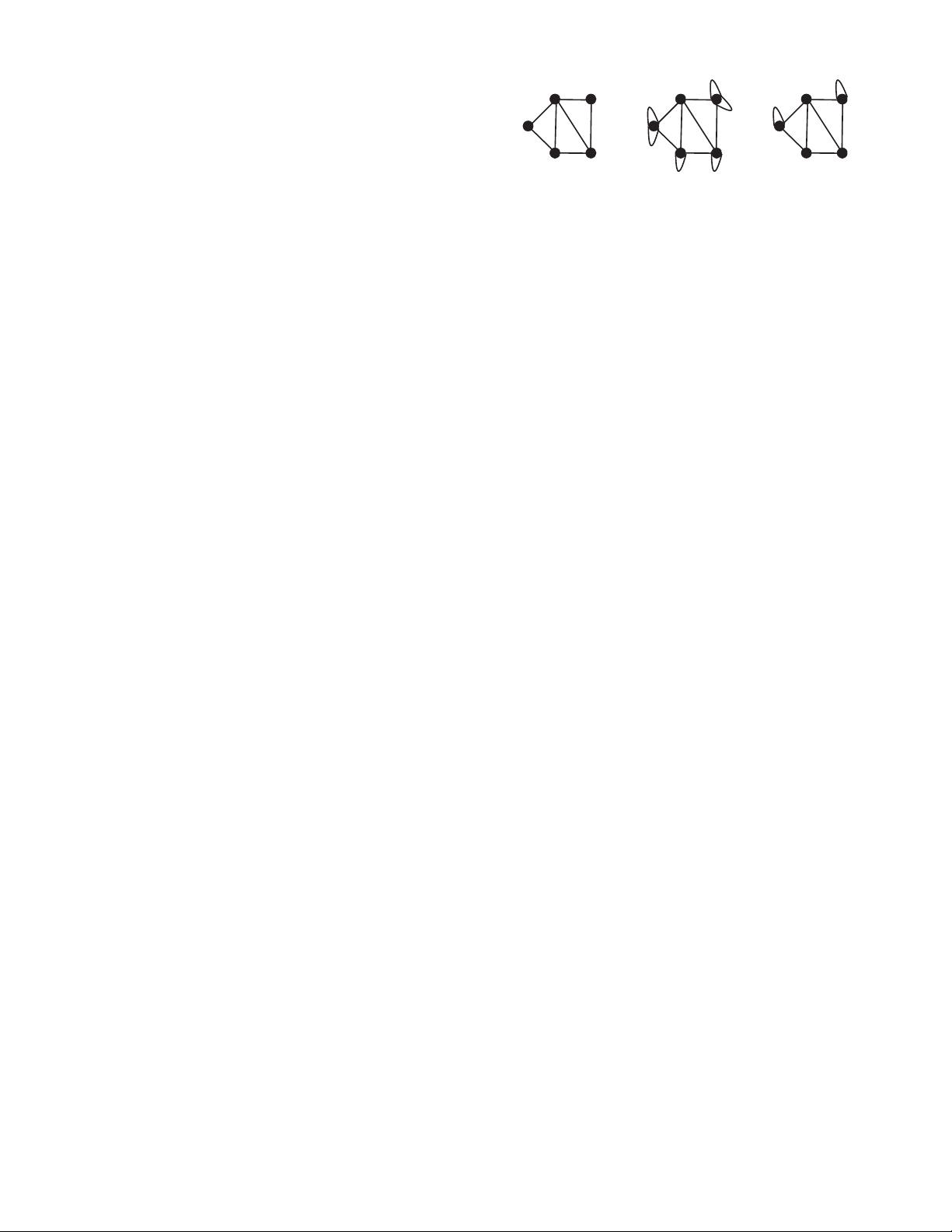
V1
V2
V3
V5
V4
(a)
V1
V2
V3
V5
V4
(b)
(c)
V1
V2
V3
V5
V4
Fig. 1: Running example
Using the language in IS framework, the trial distribution of
MH is equivalent to th e target distribution, i.e., π
u
= π
mh
.
This suggests that MH can overcome the large deviation
problem of RW. However, this is not free. To obtain the
uniform samples, MH has to reject a considerable number of
samples. In other words, to achieve the same sample size as
that of RW, MH g enerally needs to d raw a lot more nodes than
RW. In the setting o f unbiased graph sampling, the primary
costs of different algorithms are measured by the number of
nodes drawn by various algorithms [1]. If we fix the number of
nodes that different algorithms need to draw, then the number
of final samples obtained by MH is much smaller than that of
RW, which clearly degrades the performance of MH. Hence,
the MH algorithm suffers from the sample rejection problem.
Maximum-degree random walk (MD). The MD algor ithm
runs a random walk on a dynamically created regular graph to
collect nodes [7], [11]. The idea is that the algorithm modifies
the original graph into a regular graph by adding self-loops
on the nodes so that the degree of each node equals the
maximum degree of the o riginal graph . Note that this can
be done implicitly and on-the-fly. Specifically, when the walk
traverses a node u, the walk selects a neighbor node from N(u)
with probability 1/d
max
,whered
max
denotes the maximum
degree of the original graph. Following this process, in each
step, the walk stays at u with probability (d
max
− d
u
)/d
max
.
That is to say, th e walk traverses the self-loop with probability
(d
max
−d
u
)/d
max
. Fig. 1(a) and Fig. 1(b) illustrate the original
graph and the corresponding regular graph respectively. For the
graph in Fig. 1(a), the maximum degree is 4. Hence, each node
in the corresponding regular graph shown in Fig. 1(b) has a
degree of 4 including self-loops. The maximum-degree random
walk on a graph is equivalent to the traditional random walk
on the corresponding regular graph. This fact indicates that the
stationary distribution of the maximum-degree random walk is
a uniform distribution. As a result, the sample m ean obtained
by MD can be directly utilized to construct an unbiased
estimator for E
π
u
(f) [7]. Similarly, using the language in
IS framework, the trial distribution of MD is equal to the
target distribution π
u
. Therefore, MD can circumvent the large
deviation problem of RW.
MD also has its drawbacks. First, the algorithm will produce
many repeated samples, because MD needs to traverse the
self-loops. This issue worsens when the walk traverses the
low-degree nodes as these nodes must add many self-loops.
Note that too many repeated samples typically result in a large
variance for the random walk based samplers [2]. Thus, MD
suffers from the repeated samples problem. Second, MD re-
quires the knowledge of maximum degree which is impractical
in the context of unbiased graph sampling via crawling. To
overcome this problem, Bar-Yossef et al. [7] propose to set
a very large constant as the maximum degree. Clearly, this
929


