JOURNAL OF L
A
T
E
X CLASS FILES, VOL. XX, NO. XX, AUGUST 2019 5
𝐆𝐫𝐚𝐩𝐡
𝑿
𝑹𝒆𝑳𝒖 𝑹𝒆𝑳𝒖
𝐎𝐮𝐭𝐩𝐮𝐭𝐬
𝐆𝐜𝐨𝐧𝐯
…
𝐆𝐜𝐨𝐧𝐯
…
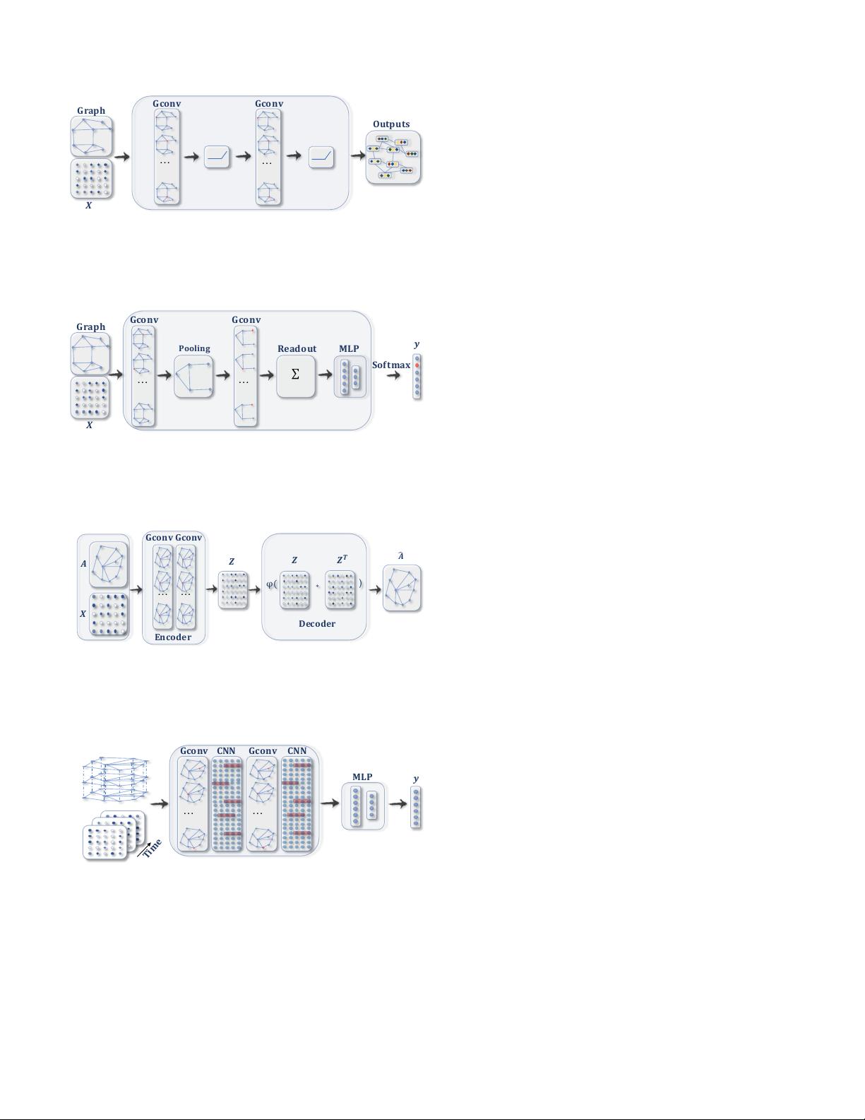
(a) A ConvGNN with multiple graph convolutional layers. A graph convo-
lutional layer encapsulates each node’s hidden representation by aggregating
feature information from its neighbors. After feature aggregation, a non-linear
transformation is applied to the resulted outputs. By stacking multiple layers,
the final hidden representation of each node receives messages from a further
neighborhood.
𝐆𝐜𝐨𝐧𝐯
𝐆𝐫𝐚𝐩𝐡
𝐑𝐞𝐚𝐝𝐨𝐮𝐭
𝐆𝐜𝐨𝐧𝐯
𝐏𝐨𝐨𝐥𝐢𝐧𝐠
𝐒𝐨𝐟𝐭𝐦𝐚𝐱
𝑿
… …
𝐌𝐋𝐏
𝒚
∑
(b) A ConvGNN with pooling and readout layers for graph classification
[21]. A graph convolutional layer is followed by a pooling layer to coarsen
a graph into sub-graphs so that node representations on coarsened graphs
represent higher graph-level representations. A readout layer summarizes the
final graph representation by taking the sum/mean of hidden representations
of sub-graphs.
𝒁"
φ (
𝒁
𝑻
𝒁
∗
)
𝑨
𝑿
𝑨
)
𝐃𝐞𝐜𝐨𝐝𝐞𝐫
𝐄𝐧𝐜𝐨𝐝𝐞𝐫
…
𝐆𝐜𝐨𝐧𝐯"𝐆𝐜𝐨𝐧𝐯
…
(c) A GAE for network embedding [61]. The encoder uses graph convolutional
layers to get a network embedding for each node. The decoder computes the
pair-wise distance given network embeddings. After applying a non-linear
activation function, the decoder reconstructs the graph adjacency matrix. The
network is trained by minimizing the discrepancy between the real adjacency
matrix and the reconstructed adjacency matrix.
𝑨
𝑿
𝐓𝐢𝐦𝐞
'''''𝐆𝐜𝐨𝐧𝐯''''𝐂𝐍𝐍''''''𝐆𝐜𝐨𝐧𝐯'''''𝐂𝐍𝐍
…
…
𝐌𝐋𝐏
𝒚
𝐓𝐢𝐦𝐞
(d) A STGNN for spatial-temporal graph forecasting [74]. A graph convolu-
tional layer is followed by a 1D-CNN layer. The graph convolutional layer
operates on A and X
(t)
to capture the spatial dependency, while the 1D-CNN
layer slides over X along the time axis to capture the temporal dependency.
The output layer is a linear transformation, generating a prediction for each
node, such as its future value at the next time step.
Fig. 2: Different graph neural network models built with
graph convolutional layers. The term Gconv denotes a graph
convolutional layer. The term MLP denotes a multi-layer
perceptron. The term CNN denotes a standard convolutional
layer.
ular way is to utilize the negative sampling approach
which samples a portion of node pairs as negative pairs
while existing node pairs with links in the graphs are
positive pairs. Then a logistic regression layer is applied
to distinguish between positive and negative pairs [42].
In Table III, we summarize the main characteristics of
representative RecGNNs and ConvGNNs. Input sources, pool-
ing layers, readout layers, and time complexity are compared
among various models. In more detail, we only compare the
time complexity of the message passing/graph convolution
operation in each model. As methods in [19] and [20] require
eigenvalue decomposition, the time complexity is O(n
3
). The
time complexity of [46] is also O(n
3
) due to the node pair-
wise shortest path computation. Other methods incur equiva-
lent time complexity, which is O(m) if the graph adjacency
matrix is sparse and is O(n
2
) otherwise. This is because in
these methods the computation of each node v
i
’s representa-
tion involves its d
i
neighbors, and the sum of d
i
over all nodes
exactly equals the number of edges. The time complexity of
several methods are missing in Table III. These methods either
lack a time complexity analysis in their papers or report the
time complexity of their overall models or algorithms.
IV. RECURRENT GRAPH NEURAL NETWORKS
Recurrent graph neural networks (RecGNNs) are mostly pi-
oneer works of GNNs. They apply the same set of parameters
recurrently over nodes in a graph to extract high-level node
representations. Constrained by computational power, earlier
research mainly focused on directed acyclic graphs [13], [80].
Graph Neural Network (GNN*
2
) proposed by Scarselli et
al. extends prior recurrent models to handle general types of
graphs, e.g., acyclic, cyclic, directed, and undirected graphs
[15]. Based on an information diffusion mechanism, GNN*
updates nodes’ states by exchanging neighborhood information
recurrently until a stable equilibrium is reached. A node’s
hidden state is recurrently updated by
h
(t)
v
=
X
u∈N(v)
f(x
v
, x
e
(v,u)
, x
u
, h
(t−1)
u
), (1)
where f(·) is a parametric function, and h
(0)
v
is initialized
randomly. The sum operation enables GNN* to be applicable
to all nodes, even if the number of neighbors differs and no
neighborhood ordering is known. To ensure convergence, the
recurrent function f(·) must be a contraction mapping, which
shrinks the distance between two points after projecting them
into a latent space. In the case of f (·) being a neural network,
a penalty term has to be imposed on the Jacobian matrix
of parameters. When a convergence criterion is satisfied,
the last step node hidden states are forwarded to a readout
layer. GNN* alternates the stage of node state propagation
and the stage of parameter gradient computation to minimize
a training objective. This strategy enables GNN* to handle
cyclic graphs. In follow-up works, Graph Echo State Network
(GraphESN) [16] extends echo state networks to improve the
2
As GNN is used to represent broad graph neural networks in the survey,
we name this particular method GNN* to avoid ambiguity.


