RBPN：视频超分辨率的循环反投影网络

下载需积分: 1 | PDF格式 | 19.85MB | 更新于2024-09-03 | 78 浏览量 | 举报

"RBPN是一种用于视频超分辨率的循环反向投影网络，由Muhammad Haris、Greg Shakhnarovich和Norimichi Ukita在2019年提出。该网络结合了空间和时间上下文，利用循环编码解码模块融合多帧信息与传统的单帧超分辨率路径，以提高目标帧的分辨率。与大多数先验工作不同，RBPN不将帧堆叠或扭曲在一起，而是将每个上下文帧视为独立的信息源。通过迭代细化框架，RBPN借鉴多图像超分辨率中的反向投影思想，并通过明确表示相对于目标帧的估计帧间运动，而非直接对齐帧，来增强信息融合。研究人员还提出了一种新的视频超分辨率基准，允许更全面的性能评估。" RBPN（Recurrent Back-Projection Network）是针对视频超分辨率问题设计的一种创新架构，其核心在于整合连续视频帧的空间和时间上下文。视频超分辨率的目标是提升低分辨率视频的质量，使其接近或达到高分辨率的清晰度。传统的视频超分辨率方法通常侧重于单帧处理，而RBPN则通过引入循环结构，能够捕捉到时间序列中的动态信息。 RBPN网络包含一个循环编码解码模块，它能有效地融合多帧信息。不同于简单地堆叠或扭曲帧来获取时间信息，RBPN对待每个帧作为一个独立的信息源，这样可以更好地捕捉帧间的差异和变化。通过这种分离处理，网络能够更精确地捕获运动信息，这对于视频处理至关重要，因为视频中的帧通常是连续且相关的。该模型的迭代细化框架受到多图像超分辨率中反向投影概念的启发。在反向投影过程中，预测的高分辨率图像被投影回低分辨率空间，以比较和校正预测误差。RBPN通过估计帧间运动并将其与目标帧的关系明确表示，而不是直接对齐帧，从而实现这一过程。这种方法减少了由于帧对齐不准确导致的失真，提高了细节恢复的准确性。此外，RBPN的作者们还贡献了一个新的视频超分辨率基准，这为研究社区提供了一个更加全面的平台，以评估和比较不同的视频超分辨率算法。这样的基准有助于推动领域的发展，促进技术的持续进步。 RBPN是视频超分辨率领域的突破性工作，通过引入循环结构和反向投影机制，有效地利用了时间信息，提高了超分辨率的效果。同时，它也促进了对视频超分辨率技术的评估和比较，对后续研究具有深远的影响。

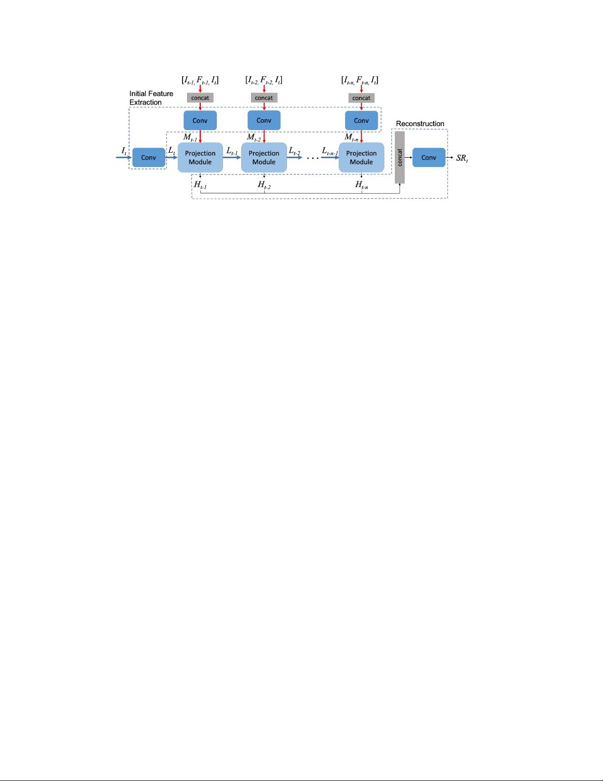
Figure 2. Overview of RBPN. The network has two approaches. The horizontal blue line enlarges I

using SISR. The vertical red line is

based on MISR to compute the residual features from a pair of I

to neighbor frames (I

t−1

, ..., I

t−n

) and the precomputed dense motion

ﬂow maps (F

t−1

, ..., F

t−n

). Each step is connected to add the temporal connection. On each projection step, RBPN observes the missing

details on I

and extract the residual features from each neighbor frame to recover the missing details.

work capacity and has no frame alignment step. Further

improvement is proposed by [30] using a motion compen-

sation module and a convLSTM layer [33]. Recently, [27]

proposed an efﬁcient many-to-many RNN that uses the pre-

vious HR estimate to super-resolve the next frames. While

recurrent feedback connections utilize temporal smoothness

between neighbor frames in a video for improving the per-

formance, it is not easy to jointly model subtle and signiﬁ-

cant changes observed in all frames.

3. Recurrent Back-Projection Networks

3.1. Network Architecture

Our proposed network is illustrated in Fig. 2. Let I be

LR frame with size of (M

× N

). The input is sequence

of n + 1 LR frames {I

t−n

, . . . , I

t−1

, I

} where I

is the

target frame. The goal of VSR is to output HR version of I

denoted by SR

with size of (M

× N

) where M

< M

and N

< N

. The operation of RBPN can be divided into

three stages: initial feature extraction, multiple projections,

and reconstruction. Note that we train the entire network

jointly, end-to-end.

Initial feature extraction. Before entering projection mod-

ules, I

is mapped to LR feature tensor L

. For each neigh-

bor frame among I

t−k

, k ∈ [n], we concatenate the pre-

computed dense motion ﬂow map F

t−k

(describing a 2D

vector per pixel) between I

t−k

and I

with the target frame

and I

t−k

. The motion ﬂow map encourages the projec-

tion module to extract missing details between a pair of I

and I

t−k

. This stacked 8-channel “image” is mapped to a

neighbor feature tensor M

t−k

Multiple Projections. Here, we extract the missing details

in the target frame by integrating SISR and MISR paths,

then produce reﬁned HR feature tensor. This stage receives

t−k−1

and M

t−k

, and outputs HR feature tensor H

t−k

Reconstruction. The ﬁnal SR output is obtained

by feeding concatenated HR feature maps for all

frames into a reconstruction module, similarly to [8]:

= f

rec

([H

t−1

, H

t−2

, ..., H

t−n

]). In our experiments,

rec

is a single convolutional layer.

3.2. Multiple Projection

The multiple projection stage of RBPN uses a re-

current chain of encoder-decoder modules, as shown in

Fig. 3. The projection module, shared across time

frames, takes two inputs: L

t−n−1

∈ R

×N

×c

and

t−n

∈ R

×N

×c

, then produces two outputs: L

t−n

and H

t−n

∈ R

×N

×c

where c

, c

are the number

of channels for particular map accordingly.

The encoder produces a hidden state of estimated HR

features from the projection to a particular neighbor frame.

The decoder deciphers the respective hidden state as the

next input for the encoder module as shown in Fig. 4 which

are deﬁned as follows:

Encoder: H

t−n

= Net

t−n−1

, M

t−n

; θ

) (1)

Decoder: L

t−n

= Net

t−n

; θ

) (2)

The encoder module Net

is deﬁned as follows:

SISR upscale: H

t−n−1

= Net

sisr

t−n−1

; θ

sisr

) (3)

MISR upscale: H

t−n

= Net

misr

t−n

; θ

misr

) (4)

Residual: e

t−n

= Net

res

t−n−1

− H

t−n

; θ

res

) (5)

Output: H

t−n

= H

t−n−1

+ e

t−n

(6)

3.3. Interpretation

Figure 5 illustrates the RBPN pipeline, for a 3-frame

video. In the encoder, we can see RBPN as the combina-

tion of SISR and MISR networks. First, target frame is en-

larged by Net

sisr

to produce H

t−k−1

. Then, for each com-

bination of concatenation from neighbor frames and target

frame, Net

misr

performs implicit frame alignment and ab-

sorbs the motion from neighbor frames to produce warping

剩余12页未读，继续阅读

FlorrieZhu

粉丝: 724

RBPN：视频超分辨率的循环反投影网络

深度学习包tree_lstm-0.0.7在PyPI官网发布

warp_rnnt-0.0.3：Python库的最新版本发布

深度学习资源包：代码实现与文档指南

Recurrent_MVSNet_for_High-Resolution_Multi-View.pdf

A-Dual-Stage-Attention-Based-Recurrent-Neural-Network-for-Time-Series-Prediction

lstm-master.rar_LSTM_LSTM-MATLAB-master_LSTM-master_lstm matlab_

Recurrent-Attention-Convolutional-Neural-Network

joone-engine-1.1.2.zip_joone_joone-engine_joone-engine.jar_神经网络

rnnoise-java-master.zip_RNN_cookiesp6x_rnnoise-java_rnnoise-java

Maggioni_Efficient_Multi-Stage_Video_CVPR_2021_supplemental.pdf

最新资源