LeNet5深度学习手写字符识别论文解析

需积分: 11 49 浏览量更新于2024-07-16 1 收藏 989KB PDF 举报

"Lecun98.pdf" 这篇论文"Gradient-Based Learning Applied to Document Recognition"由Yann LeCun、Leon Bottou、Yoshua Bengio和Patrick Haffner共同撰写，详细介绍了LeNet5，这是一个经典的卷积神经网络（CNN）架构，用于文档识别，特别是手写字符识别。论文主要探讨了基于梯度的学习方法在处理高维模式分类问题中的应用，如手写字符的识别。 LeNet5是最早成功应用反向传播算法训练的多层神经网络之一，它能构建复杂的决策表面，对未经大量预处理的高维模式进行有效分类。论文回顾了多种手写字符识别的方法，并在标准的手写数字识别任务上进行了比较。其中，卷积神经网络由于其特殊的设计，能够处理形状变化的多样性，表现优于其他技术。在实际的文档识别系统中，除了LeNet5这样的模型之外，还包括多个模块，如字段提取、图像预处理、特征提取等。这些模块协同工作，以实现高效且准确的文档自动化处理。LeNet5的核心在于其卷积层和池化层，它们能够捕捉局部特征并减少数据的维度，同时保持关键信息。此外，论文还讨论了权值共享的概念，这是卷积网络的一个重要特性，可以显著减少模型参数数量，提高计算效率，并增强模型的泛化能力。 LeNet5的成功开启了深度学习在图像识别领域的广泛应用，为后来的AlexNet、VGG、ResNet等更先进的网络架构奠定了基础。通过不断的优化和改进，这些网络在图像分类、物体检测、语义分割等多个任务上取得了前所未有的性能。这篇论文不仅在技术上具有里程碑意义，而且对整个机器学习和计算机视觉领域的发展产生了深远的影响。

PROC. OF THE IEEE, NOVEMBER 1998 8

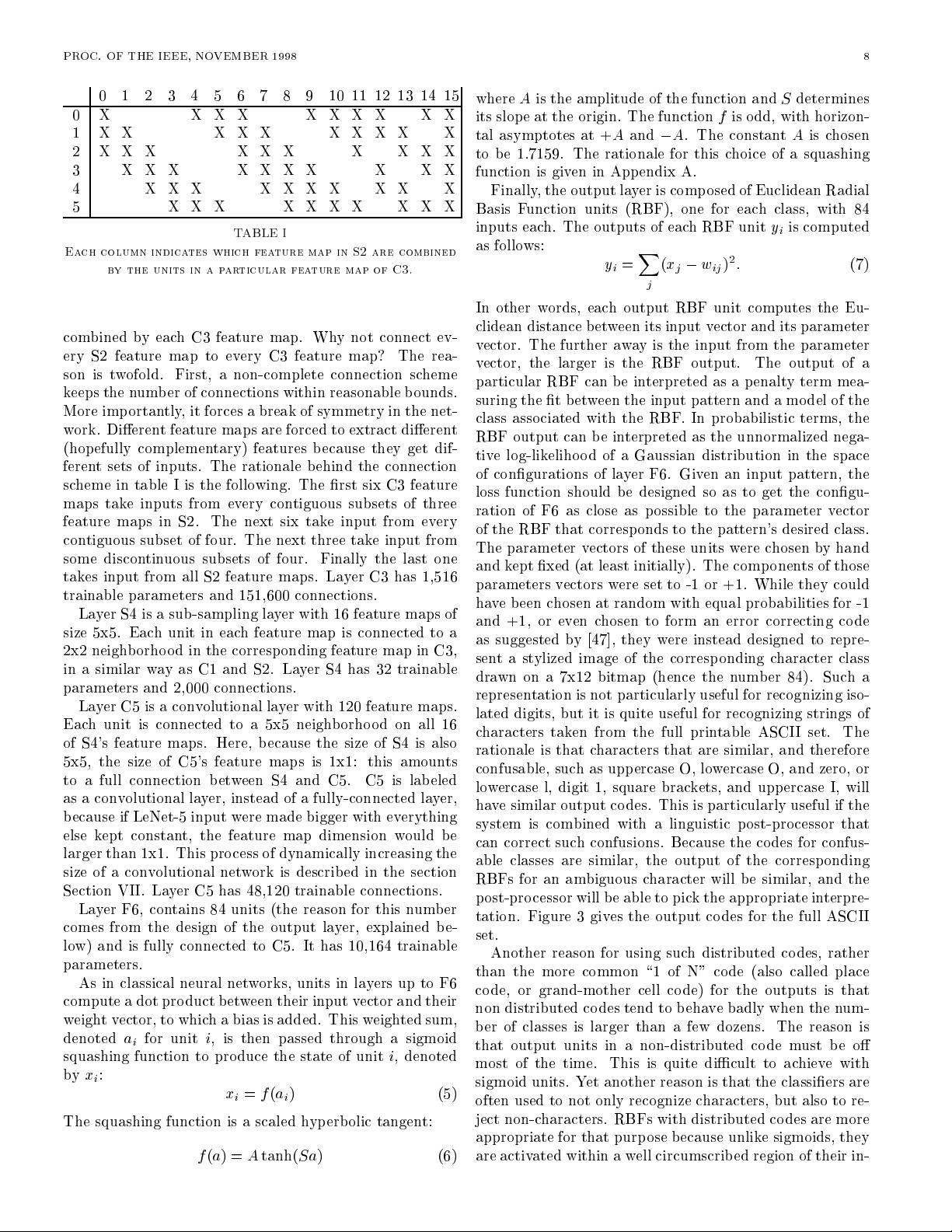
0 1 2 3 4 5 6 7 8 9 10 11 12 13 14 15

0 X X X X X X X X X X

1 X X X X X X X X X X

2 X X X X X X X X X X

3 X X X X X X X X X X

4 X X X X X X X X X X

5 X X X X X X X X X X

TABLE I

Each column indicates which feature map in S2 are combined

by the units in a particular feature map of C3.

combined byeach C3 feature map. Why not connect ev-

ery S2 feature map to every C3 feature map? The rea-

son is twofold. First, a non-complete connection scheme

keeps the numb er of connections within reasonable bounds.

More importantly, it forces a break of symmetry in the net-

work. Dierent feature maps are forced to extract dierent

(hopefully complementary) features b ecause they get dif-

ferent sets of inputs. The rationale behind the connection

scheme in table I is the following. The rst six C3 feature

maps take inputs from every contiguous subsets of three

feature maps in S2. The next six take input from every

contiguous subset of four. The next three take input from

some discontinuous subsets of four. Finally the last one

takes input from all S2 feature maps. Layer C3 has 1,516

trainable parameters and 151,600 connections.

Layer S4 is a sub-sampling layer with 16 feature maps of

size 5x5. Eachunitineach feature map is connected to a

2x2 neighb orhood in the corresponding feature map in C3,

in a similar way as C1 and S2. Layer S4 has 32 trainable

parameters and 2,000 connections.

Layer C5 is a convolutional layer with 120 feature maps.

Each unit is connected to a 5x5 neighborhood on all 16

of S4's feature maps. Here, because the size of S4 is also

5x5, the size of C5's feature maps is 1x1: this amounts

to a full connection between S4 and C5. C5 is labeled

as a convolutional layer, instead of a fully-connected layer,

because if LeNet-5 input were made bigger with everything

else kept constant, the feature map dimension would be

larger than 1x1. This process of dynamically increasing the

size of a convolutional network is describ ed in the section

Section VI I. Layer C5 has 48,120 trainable connections.

Layer F6, contains 84 units (the reason for this number

comes from the design of the output layer, explained be-

low) and is fully connected to C5. It has 10,164 trainable

parameters.

As in classical neural networks, units in layers up to F6

compute a dot pro duct between their input vector and their

weightvector, to whichabiasisadded. This weighted sum,

denoted

for unit

, is then passed through a sigmoid

squashing function to produce the state of unit

, denoted

(

) (5)

The squashing function is a scaled hyperbolic tangent:

(

tanh(

) (6)

where

is the amplitude of the function and

determines

its slop e at the origin. The function

is o dd, with horizon-

tal asymptotes at +

and

;

. The constant

is chosen

to b e 1

7159. The rationale for this choice of a squashing

function is given in Appendix A.

Finally, the output layer is composed of Euclidean Radial

Basis Function units (RBF), one for each class, with 84

inputs each. The outputs of each RBF unit

is computed

as follows:

(

;

)

(7)

In other words, each output RBF unit computes the Eu-

clidean distance b etween its input vector and its parameter

vector. The further away is the input from the parameter

vector, the larger is the RBF output. The output of a

particular RBF can b e interpreted as a penalty term mea-

suring the t between the input pattern and a mo del of the

class associated with the RBF. In probabilistic terms, the

RBF output can b e in

terpreted as the unnormalized nega-

tive log-likeliho od of a Gaussian distribution in the space

of congurations of layer F6. Given an input pattern, the

loss function should b e designed so as to get the congu-

ration of F6 as close as p ossible to the parameter vector

of the RBF that corresponds to the pattern's desired class.

The parameter vectors of these units were chosen byhand

and kept xed (at least initially). The components of those

parameters vectors were set to -1 or +1. While they could

have been chosen at random with equal probabilities for -1

and +1, or even chosen to form an error correcting co de

as suggested by 47], they were instead designed to repre-

sentastylized image of the corresp onding character class

drawn on a 7x12 bitmap (hence the number 84). Such a

representation is not particularly useful for recognizing iso-

lated digits, but it is quite useful for recognizing strings of

characters taken from the full printable ASCI I set. The

rationale is that characters that are similar, and therefore

confusable, suchasuppercaseO,lowercase O, and zero, or

lowercase l, digit 1, square brackets, and uppercase I, will

ve similar output codes. This is particularly useful if the

system is combined with a linguistic p ost-processor that

can correct such confusions. Because the codes for confus-

able classes are similar, the output of the corresponding

RBFs for an ambiguous character will b e similar, and the

post-pro cessor will b e able to pick the appropriate interpre-

tation. Figure 3 gives the output codes for the full ASCI I

set.

Another reason for using such distributed co des, rather

than the more common \1 of N" co de (also called place

code, or grand-mother cell code) for the outputs is that

non distributed codes tend to behave badly when the num-

ber of classes is larger than a few dozens. The reason is

that output units in a non-distributed co de must be o

most of the time. This is quite dicult to achieve with

sigmoid units. Yet another reason is that the classiers are

often used to not only recognize c

haracters, but also to re-

ject non-characters. RBFs with distributed codes are more

appropriate for that purp ose b ecause unlike sigmoids, they

are activated within a well circumscrib ed region of their in-

PROC. OF THE IEEE, NOVEMBER 1998 9

! " # $ % & ’ ( ) * + , − . /

0 1 2 3 4 5 6 7 8 9 : ; < = > ?

@ A B C D E F G H I J K L M N O

P Q R S T U V W X Y Z [ \ ] ^ _

‘ a b c d e f g h i j k l m n o

p q r s t u v w x y z { | } ~

Fig. 3. Initial parameters of the output RBFs for recognizing the

full ASCI I set.

put space that non-typical patterns are more likely to fall

outside of.

The parameter vectors of the RBFs play the role of target

vectors for layer F6. It is worth pointing out that the com-

ponents of those vectors are +1 or -1, whichiswell within

the range of the sigmoid of F6, and therefore prevents those

sigmoids from getting saturated. In fact, +1 and -1 are the

points of maximum curvature of the sigmoids. This forces

the F6 units to op erate in their maximally non-linear range.

Saturation of the sigmoids must be avoided b ecause it is

known to lead to slow convergence and ill-conditioning of

the loss function.

C. Loss Function

The simplest output loss function that can be used with

the ab ovenetwork is the Maximum Likeliho od Estimation

criterion (MLE), which in our case is equivalent to the Min-

imum Mean Squared Error (MSE). The criterion for a set

of training samples is simply:

(

W

) (8)

where

is the output of the

-th RBF unit, i.e. the

one that corresp onds to the correct class of input pattern

. While this cost function is appropriate for most cases,

it lacks three imp ortant properties. First, if weallowthe

parameters of the RBF to adapt,

(

) has a trivial, but

totally unacceptable, solution. In this solution, all the RBF

parameter vectors are equal, and the state of F6 is constant

and equal to that parameter vector. In this case the net-

work happily ignores the input, and all the RBF outputs

are equal to zero. This collapsing phenomenon do es not

occur if the RBF weights are not allowed to adapt. The

second problem is that there is no competition between

the classes. Suc

h a competition can be obtained by us-

ing a more discriminative training criterion, dubbed the

MAP (maximum a p osteriori) criterion, similar to Maxi-

mum Mutual Information criterion sometimes used to train

HMMs 48], 49], 50]. It corresp onds to maximizing the

posterior probability of the correct class

(or minimiz-

ing the logarithm of the probabilityofthe correct class),

given that the input image can come from one of the classes

or from a background \rubbish" class lab el. In terms of

penalties, it means that in addition to pushing down the

penalty of the correct class like the MSE criterion, this

criterion also pulls up the penalties of the incorrect classes:

(

W

) + log(

;

(

W

)

))

(9)

The negative of the second term plays a \comp etitive" role.

It is necessarily smaller than (or equal to) the rst term,

therefore this loss function is positive. The constant

positive, and prevents the penalties of classes that are al-

ready very large from b eing pushed further up. The p os-

terior probabilityofthis rubbish class lab el would be the

ratio of

;

and

;

(

W

)

. This discrimina-

tive criterion prevents the previously mentioned \collaps-

ing eect" when the RBF parameters are learned because

it keeps the RBF centers apart from each other. In Sec-

tion VI, we present a generalization of this criterion for

systems that learn to classify multiple ob jects in the input

(e.g., characters in words or in do cuments).

Computing the gradient of the loss function with respect

to all the weights in all the layers of the convolutional

network is done with back-propagation. The standard al-

gorithm must be slightly mo died to take accountofthe

weight sharing. An easy way to implement it is to rst com-

pute the partial derivatives of the loss function with resp ect

to each

connection

, as if the network were a conventional

multi-layer network without weight sharing. Then the par-

tial derivatives of all the connections that share a same

parameter are added to form the derivative with respect to

that parameter.

Such a large architecture can b e trained very eciently,

but doing so requires the use of a few techniques that are

described in the app endix. Section A of the app endix

describes details such as the particular sigmoid used, and

the weight initialization. Section B and C describe the

minimization procedure used, whichisastochastic version

of a diagonal approximation to the Levenberg-Marquardt

procedure.

III. Results and Comparison with Other

Methods

While recognizing individual digits is only one of many

problems involved in designing a practical recognition sys-

tem, it is an excellent benchmark for comparing shape

recognition methods. Though many existing method com-

bine a hand-crafted feature extractor and a trainable clas-

sier, this study concentrates on adaptive metho ds that

operate directly on size-normalized images.

A. Database: the ModiedNISTset

The

database used to train and test the systems de-

scribed in this paper was constructed from the NIST's Spe-

cial Database 3 and Special Database 1 containing binary

images of handwritten digits. NIST originally designated

SD-3 as their training set and SD-1 as their test set. How-

ever, SD-3 is much cleaner and easier to recognize than SD-

1. The reason for this can b e found on the fact that SD-3

PROC. OF THE IEEE, NOVEMBER 1998 10

was collected among Census Bureau employees, while SD-1

was collected among high-school students. Drawing sensi-

ble conclusions from learning experiments requires that the

result be indep endent of the choice of training set and test

among the complete set of samples. Therefore it was nec-

essary to build a new database by mixing NIST's datasets.

SD-1 contains 58,527 digit images written by 500 dif-

ferent writers. In contrast to SD-3, where blocks of data

from each writer appeared in sequence, the data in SD-1 is

scrambled. Writer identities for SD-1 are available and we

used this information to unscramble the writers. Wethen

split SD-1 in two: characters written by the rst 250 writers

wentinto our new training set. The remaining 250 writers

were placed in our test set. Thus we had two sets with

nearly 30,000 examples each. The new training set was

completed with enough examples from SD-3, starting at

pattern # 0, to make a full set of 60,000 training patterns.

Similarly, the new test set was completed with SD-3 exam-

ples starting at pattern # 35,000 to makeafull set with

60,000 test patterns. In the exp eriments describ ed here, we

only used a subset of 10,000 test images (5,000 from SD-1

and 5,000 from SD-3), but we used the full 60,000 training

samples. The resulting database was called the Mo died

NIST, or MNIST, dataset.

The original black and white (bilevel) images were size

normalized to t in a 20x20 pixel box while preserving

their asp ect ratio. The resulting images contain grey lev-

els as result of the anti-aliasing (image interpolation) tech-

nique used by the normalization algorithm. Three ver-

sions of the database were used. In the rst version,

the images were centered in a 28x28 image by comput-

ing the center

of mass of the pixels, and translating the

image so as to position this point at the center of the

28x28 eld. In some instances, this 28x28 eld was ex-

tended to 32x32 with background pixels. This version of

the database will be referred to as the

regular

database.

In the second version of the database, the character im-

ages were deslanted and cropped down to 20x20 pixels im-

ages. The deslanting computes the second moments of in-

ertia of the pixels (counting a foreground pixel as 1 and a

background pixel as 0), and shears the image by horizon-

tally shifting the lines so that the principal axis is verti-

cal. This version of the database will b e referred to as the

deslanted

database. In the third

version of the database,

used in some early exp eriments, the images were reduced

to 16x16 pixels. The regular database (60,000 training

examples, 10,000 test examples size-normalized to 20x20,

and centered by center of mass in 28x28 elds) is avail-

able at

http://www.research.att.com/

yann/ocr/mnist

Figure 4 shows examples randomly picked from the test set.

B. Results

Several versions of LeNet-5 were trained on the regular

MNIST database. 20 iterations through the entire train-

ing data were p erformed for each session. The values of

the global learning rate



(see Equation 21 in App endix C

for a denition) was decreased using the following sched-

ule:

0.0005 for the rst two passes, 0.0002 for the next

Fig. 4. Size-normalized examples from the MNIST database.

three, 0.0001 for the next three, 0.00005 for the next 4,

and 0.00001 thereafter. Before each iteration, the diagonal

Hessian approximation was reevaluated on 500 samples, as

described in App endix C and kept xed during the entire

iteration. The parameter



wassetto0.02. The resulting

eective learning rates during the rst pass varied between

approximately 7



;

and 0

016 over the set of parame-

ters. The test error rate stabilizes after around 10 passes

through the training set at 0.95%. The error rate on the

training set reaches 0.35% after 19 passes. Many authors

have reported observing the common phenomenon of over-

training when training neural networks or other adaptive

algorithms on various tasks. When over-training occurs,

the training error keeps decreasing over time, but the test

error go es through a minimum and starts increasing after

a certain number of iterations. While this phenomenon is

very common, it was not observed in our case as the learn-

ing curves in gure 5 show. A possible reason is that the

learning rate was k

ept relatively large. The eect of this is

that the weights never settle down in the lo cal minimum

but keep oscillating randomly. Because of those uctua-

tions, the average cost will be lower in a broader minimum.

Therefore, stochastic gradient will have a similar eect as

a regularization term that favors broader minima. Broader

minima corresp ond to solutions with large entropyofthe

parameter distribution, which is benecial to the general-

ization error.

The inuence of the training set size was measured by

training the network with 15,000, 30,000, and 60,000 exam-

ples. The resulting training error and test error are shown

in gure 6. It is clear that, even with specialized architec-

tures such as LeNet-5, more training data would improve

the accuracy.

Toverify this hypothesis, we articially generated more

training examples by randomly distorting the original

training images. The increased training set was composed

of the 60,000 original patterns

plus 540,000 instances of

剩余45页未读，继续阅读

*逍遥*

粉丝: 32
资源: 10

LeNet5深度学习手写字符识别论文解析

深度学习经典论文解析与链接

2023智源大会：悟道3.0全面开源，LeCun与Max精彩演讲亮点

LeNet论文解析：CNN架构的开创性研究

Lecun1998.pdf

70页《自监督学习》最新简明指南，图灵奖LeCun等编著 .pdf

谷歌：CNN击败Transformer，有望成为预训练界新霸主！LeCun却沉默了.._.pdf

NatureDeepReview(Yann LeCun+Yoshua Bengio+Geoffrey Hinton).pdf

悟道3.0全面开源！LeCun VS Max 智源大会最新演讲.pdf

Yann LeCun 新作！大幅超越 MAE，图像语义表示卷出新高度.pdf

LeCun：ChatGPT无法实现通用人工智能，但ALM技术路线可以！.pdf

最新资源