3410 IEEE TRANSACTIONS ON SIGNAL PROCESSING, VOL. 61, NO. 13, JULY 1, 2013
(18)
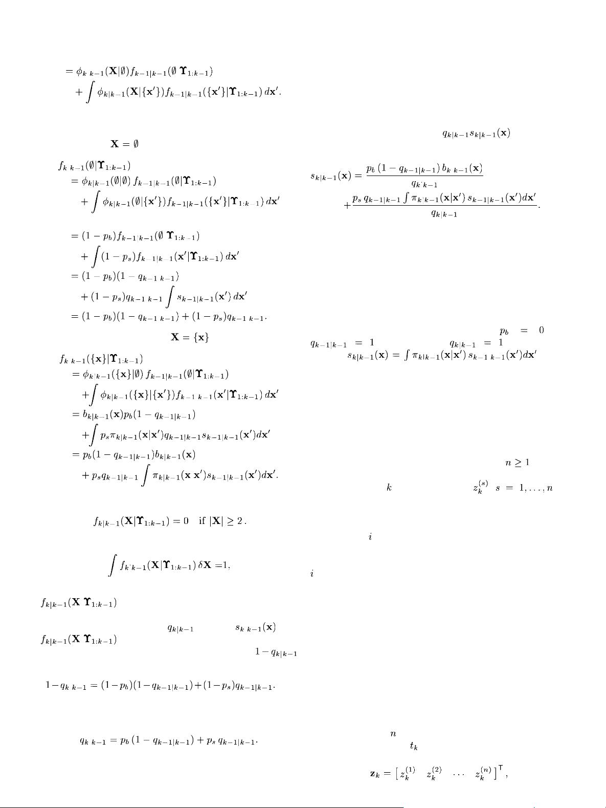
Equation (18) follows from (17) using (13). Let u s first solve
(18) for the case
. Using (16) we have:
(19)
(20)
(21)
(22)
Next we solv e (18) for the case
. Using (16) we have:
(23)
(24)
(25)
Additionally we have from (18) and (16) that:
(26)
Hence we can easily verify that
and by comparing with (7) we have established that
is a FISST probability density for a
Bernoulli RFS.
Next we solve for
and of
. Since the predicted FISST PD F is
in the form (7), then the left-hand side of (22) equals
and we can write (22) as:
(27)
This leads to the prediction equation for the probability of
existence:
(28)
Notice that (28) has an intuit ive interpretatio n. Loosely
speaking, it states that a predicted target can arise from a new
birth o r an existing survival. The predicted existence proba-
bility consist of two additive terms: the probability of t arget
non-existence and target birth, and the probability of target
existence and survival.
Similarly, since the predicted FISST PDF is in the form of (7),
the left-hand side of (25) equals
.Thisleadsto
the upd ate equation for th e spatial PDF of the Bernoulli filter:
(29)
Notice also that (29) h as an intuitive interpretatio n. Loosely
speaking, it states that the probability den sity of the predicted
state comprises a birth component and a surviving compon ent.
The birth component is the birth density weighted by the proba-
bility of target non-existence and new birth. The surviving com-
ponent com prises the standard Chap man –Ko lm ogorov predic-
tion weighted by the probability of target existence and su rvival.
Equation (28) and (29) f ully specify the prediction
step of the Bernoulli filter. Not e that if
,and
, then f rom (28) while (29) re-
duces to
,which
is the standard Chapman-Kolm og oro v prediction given by (3).
In the next three sections we wi ll present the update equations
of the Bernoulli filter for different measurement models.
IV. I
NTENSITY MEASUREMENTS
A. Intensity Measurement M odel
Suppose the sensor at our disposal consist of
intensity
measuring elements at known locations, each reporting instan-
taneously at tim e
a m easured value , .In
this (fairly general) formulation, an element can be one of the
following.
A Pixels of an Image: For a monochromatic image, the
value in pix el
can be a measure of reflective light or tempera-
ture. For a color image, it can be a measure of the similarity be-
tween the color histog ram computed in a box centered at pixel
and a reference histogram [35].
A bin in a Range-Doppler-Azimuth Map: This correspo nds
to the radar context [36], where intensity of a bin refers to the
electromagnetic energy gathered in a resolution volume of the
corresponding range-Doppler-azimuth cell.
A Node in a Sensor Network: The assumption is that all
sensor nodes sample the environment synchronously. Intensity
in this context depends on the purpose of the sensor network
— it can refer to the level of pollution (for a chem ical sensor
network), radiation (for a network of Geiger-M üller counters),
or acoustic energy (for an array of m icroph ones). Note that the
placement of nodes in the sensor network can be arbitrary, as
long as their locations are known.
We can stack all
measurements into a single m easurem ent
vector collected at time
:
(30)


