深度学习领域卷积神经网络全览：历史、模型进展与未来趋势

需积分: 50 4 浏览量更新于2024-07-16 2 收藏 3.7MB PDF 举报

本文是一篇深度探讨卷积神经网络（Convolutional Neural Network, CNN）的21页全面综述论文。CNN作为深度学习领域的重要组成部分，在计算机视觉、自然语言处理等领域取得了显著成果，近年来吸引了产业界和学术界的广泛关注。作者在本研究中超越了现有的主要关注应用层面的文献，力求从更广阔的视角出发，提供新的理论见解和未来发展趋势。论文首先回顾了CNN的历史，强调了其从早期概念到现代技术的演变过程，以及关键里程碑事件。通过对CNN历史的梳理，读者可以更好地理解这一领域的发展脉络和重要转折点。接着，论文深入解析了CNN的基本原理和架构，包括滤波器的使用、特征检测和池化层的作用，以及权重共享等核心特性。这有助于读者掌握CNN的核心计算机制。然后，文章详细介绍了经典和先进的CNN模型，重点突出了这些模型在达到当前最高性能时的关键设计元素和技术突破。这些模型分析涵盖了诸如ResNet、Inception、VGG等知名网络，以及它们在特定任务中的优化策略和改进方法。通过实验分析，论文提出了一些关于模型选择和实践中的经验法则，帮助读者理解如何根据具体应用场景有效地调整和优化CNN。这包括如何平衡模型复杂度与性能，以及如何处理过拟合等问题。文章进一步扩展到了一维、二维和多维卷积的讨论，展现了CNN在不同数据维度上的通用性和灵活性。例如，一维CNN在文本分类中的应用，二维CNN在图像识别中的应用，以及多维卷积在网络如3D医学影像分析中的应用。最后，论文指出了CNN面临的挑战和未来的研究方向，包括但不限于网络效率、迁移学习、自适应卷积、对抗性攻击防御等议题。这些前沿话题为后续的研究者提供了宝贵的启示和潜在的研究课题。这篇综述论文为读者提供了一个全面且深入的CNN框架，旨在帮助读者理解和应用这种强大的机器学习工具，同时也激发他们在该领域的创新思维。无论是初学者还是研究者，都能从中获取有价值的知识和洞见，推动该领域不断向前发展。

> REPLACE THIS LINE WITH YOUR PAPER IDENTIFICATION NUMBER (DOUBLE-CLICK HERE TO EDIT) <

block are narrower than the middle. Using 1 × 1 convolution

kernel can not only reduce the number of parameters in the

network but also greatly improve the network's nonlinearity.

A lot of experiments in [37] have proved that ResNet can

mitigate the gradient vanishing problem without degeneration

in deep neural networks since the gradient can directly flow

through shortcut connections.

Based upon ResNet, many studies have managed to improve

the performance of the original ResNet, such as pre-activation

ResNet [38], wide ResNet [39], stochastic depth ResNets (SDR)

[40], and ResNet in ResNet (RiR) [41].

F. DCGAN

Generative Adversarial Network (GAN) [42] is an

unsupervised model proposed by Goodfellow et al. in 2014.

GAN contains a generative model G and a discriminative model

D. The model G with random noise z generates a sample G(z)

that subjects to the data distribution P

data

learned by G. The

model D can determine whether the input sample is real data x

or generated data G(z). Both G and D can be nonlinear functions,

such as deep neural networks. The aim of G is to generate data

as real as possible; nevertheless, the aim of D is to distinguish

the fake data generated by G from the real data. There exists an

interestingly adversarial relationship between the generative

network and the discriminative network. This idea originates

from game theory, in which the two sides use their strategies to

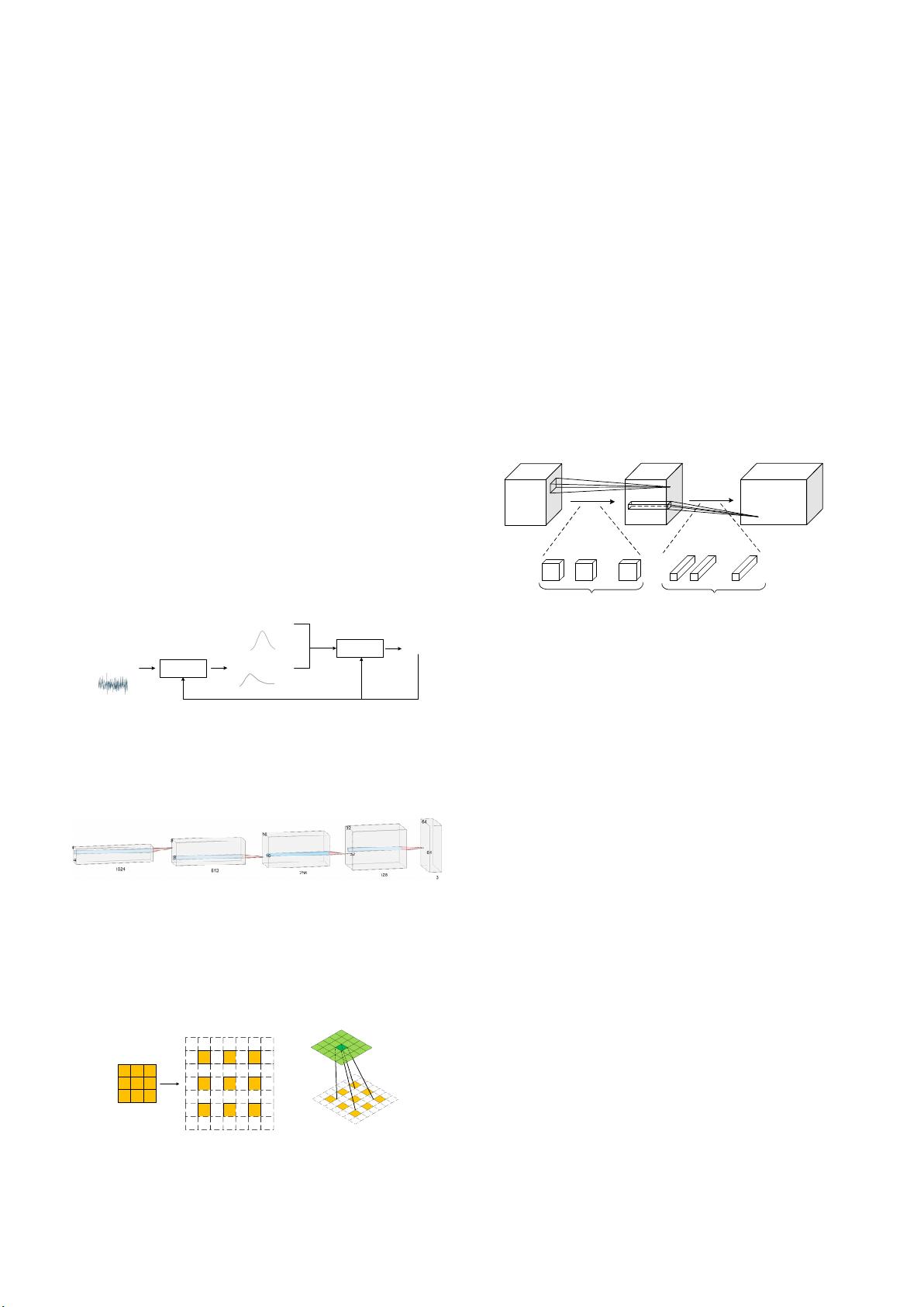
achieve the goal of winning. The procedure is shown in Fig. 10.

Radford et al. [43] proposed Deep Convolutional Generative

Adversarial Network (DCGAN) in 2015. The generator of

DCGAN on Large-scale Scene Understanding (LSUN) dataset

is implemented by using deep convolutional neural networks,

the structure of which is shown in the figure below.

In Fig. 11, the generative model of DCGAN performs up-

sampling by "fractionally-strided convolution". As shown in

Fig. 12 (a), supposing that there is a 3 × 3 input, and the size of

the output is expected to be larger than 3 × 3, then the 3 × 3

input can be expanded by inserting zero between pixels. After

expanding to a 5 × 5 size, performing convolution, shown in

Fig. 12 (b), can obtain an output larger than 3 × 3.

G. MobileNets

MobileNets are a series of lightweight models proposed by

Google for embedded devices such as mobile phones. They use

depth-wise separable convolutions and several advanced

techniques to build thin deep neural networks. There are three

versions of MobileNets to date, namely MobileNet v1 [44],

MobileNet v2 [45], and MobileNet v3 [46].

1) MobileNet v1

MobileNet v1 [44] utilizes depth-wise separable convolutions

proposed in Xception [26], which decomposes the standard

convolution into depth-wise convolution and pointwise

convolution (1 × 1 convolution), as shown in Fig. 13.

Specifically, standard convolution applies each convolution

kernel to all the channels of input. In contrast, depth-wise

convolution applies each convolution kernel to only one

channel of input, and then 1 × 1 convolution is used to combine

the output of depth-wise convolution. This decomposition can

substantially reduce the number of parameters.

MobileNet v1 also introduces the width multiplier to reduce

the number of channels of each layer and the resolution

multiplier to lower the resolution of the input image (feature

map).

2) MobileNet v2

Based upon MobileNet v1, MobileNet v2 [45] mainly

introduces two improvements: inverted residual blocks and

linear bottleneck modules.

In Section 3.5, we have explained three-layer residual blocks,

the purpose of which is to make use of 1 × 1 convolution to

reduce the number of parameters involved in 3 × 3 convolution.

In a word, the whole process of a residual block is channel

compression—standard convolution—channel expansion. In

MobileNet v2, an inverted residual block (seen in Fig. 14 (b))

is opposite to a residual block (seen in Fig. 14 (a)). The input of

an inverted residual block is firstly convoluted by 1 × 1

convolution kernels for channel expansion, then convoluted by

3 × 3 depth-wise separable convolution, and finally convoluted

by 1 × 1 convolution kernels to compress the number of

channels back. Briefly speaking, the whole process of an

inverted residual block is channel expansion—depth-wise

separable convolution—channel compression. Also, due to the

fact that depth-wise separable convolution cannot change the

number of channels, which causes the number of input channels

limits the feature extraction, inverted residual blocks are

harnessed to handle the problem.

Generator

Discriminator

Real data x

Generated data G(z)Random noise z

Result [0, 1]

Update

Fig. 10. The flowchart of GAN

Fig. 11. DCGAN generator used for LSUN scene modeling

(a) (b)

Fig. 12. An example of fractionally-strided

convolution. (a) Inserting zero

between 3 × 3 kernel points. (b) Convolving the 7 × 7 graph

#M, d×d×1

#N, 1×1×M

...

M N

...

Fig. 13. Depth-

wise separable convolutions in MobileNet v1. #M and #N

represent the number of kernels of depth-wise convolution and po

intwise

convolution, respectively

剩余20页未读，继续阅读

syp_net

粉丝: 159
资源: 1187

深度学习领域卷积神经网络全览：历史、模型进展与未来趋势

卷积神经网络结构原理详细介绍

卷积神经网络(CNN)的17篇有影响力的论文题目和创新点介绍

卷积神经网络英文版综述

基于深度学习的行人检测和行人重识别研究与应用(毕设&课设论文参考).pdf

深度学习在高光谱图像分类领域的研究现状与展望.pdf

2019-2021数学中国网络挑战赛优秀论文-2019-2021数学中国网络挑战赛优秀论文汇总-2718队A题.pdf

论文研究-运动目标跟踪算法研究综述.pdf

我国气象领域应用人工智能技术的现状和国际对比.pdf

深度学习在无人驾驶汽车领域应用的研究进展.pdf

selectiveSearchDraft.pdf

最新资源