生物启发的视觉场景识别框架：模板匹配与最大池化结合

需积分: 12 76 浏览量更新于2024-07-31 收藏 3.49MB PDF 举报

"Robust Object Recognition with Cortex-Like Mechanisms"是一篇深入探讨生物启发式计算机视觉方法的论文。作者Thomas Serre、Lior Wolf、Stanley Bileschi、Maximilian Riesenhuber和Tomaso Poggio（IEEE会员）提出了一种新的物体识别框架，灵感来源于大脑视觉皮层的结构。他们设计了一个层次化的系统，该系统模仿了视觉皮层的组织，通过交替运用模板匹配和最大池化操作，构建出复杂且不变性的特征表示。在这个框架中，系统首先进行模板匹配，通过检测场景中的特定模式或对象来定位和识别。然后，通过最大池化操作，系统能够处理尺度变化、旋转和部分遮挡等变异性问题，提高了对复杂视觉场景的理解能力。这种机制使得模型能够在单个物体识别、混杂环境下的目标检测，以及涉及形状和纹理的多类分类任务中展现出强大的性能。值得注意的是，这个生物约束驱动的方法具有从少量训练样本中学习的能力，这在数据稀缺的情况下尤为关键。它在与当时最先进的系统竞争中表现出令人惊讶的效果，证明了其在实际应用中的有效性。论文还探讨了存在一个通用且冗余的特征字典的可能性，这个字典可以处理大多数物体类别，进一步扩展了模型的泛化能力。 "Robust Object Recognition with Cortex-Like Mechanisms"为计算机视觉领域提供了一个新的视角，展示了如何通过模拟人脑处理视觉信息的方式，实现更加鲁棒和高效的物体识别。这篇研究不仅提升了人工智能在复杂场景中的表现，也为我们理解生物智能和机器学习之间的联系提供了有价值的洞察。

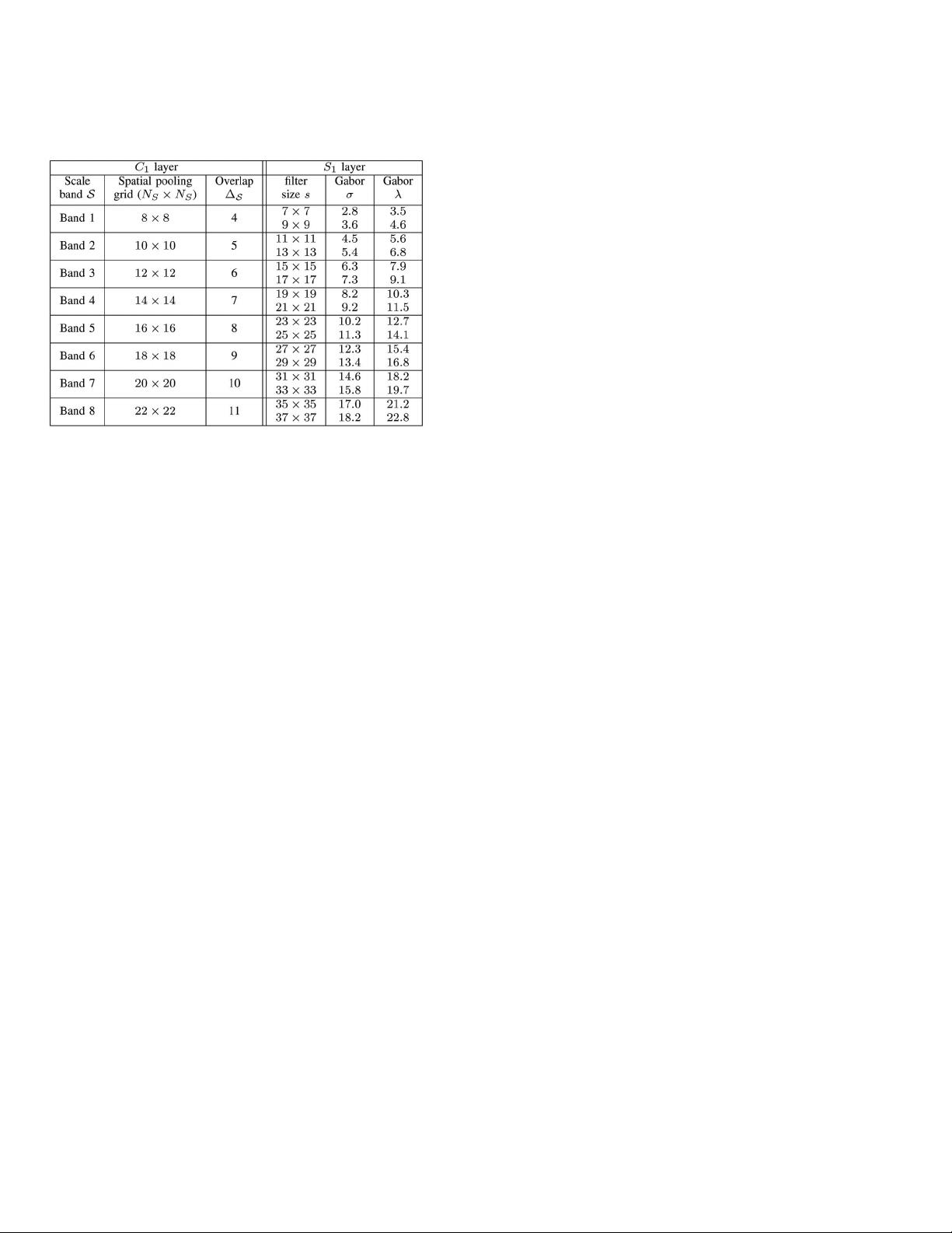
only the maximum value from the two maps. Note that

responses are not computed at every possible locations

and that C

units only overlap by an amount 

. This makes

the computations at the next stage more efficient. Again,

parameters (see Table 1) governing this pooling operation

were adjusted such that the tuning of the C

units match the

tuning of complex cells as measured experimentally (see [41]

for details).

units: In the S

layer, units pool over afferent C

units

from a local spatial neighborhood across all four orienta-

tions. S

units behave as radial basis function ( RBF) units.

Each S

unit response depends in a Gaussian-like way on

the Euclidean distance between a new input and a stored

prototype. That is, for an image patch X from the previous

layer at a particular scale S, the response r of the

corresponding S

unit is given by:

r ¼ exp kX  P



; ð4Þ

where  defines the sharpness of the

TUNING and P

is one

of the N features (center of the

RBF units) learned during

training (see below). At runtime, S

maps are computed

across all positions for each of the eight scale bands. One

such multiple scale map is computed for each one of the

ðN  1; 000Þ prototypes P

units: Our final set of shift- and scale-invariant C

responses is computed by taking a global maximum ((3))

over all scales and positions for each S

type over the entire

lattice, i.e., the S

measures the match between a stored

prototype P

and the input image at every position and

scale; we only keep the value of the best match and discard

the rest. The result is a vector of NC

values, where N

corresponds to the number of prototypes extracted during

the learning stage.

The learning stage: The learning process corresponds to

selecting a set of N prototypes P

(or features) for the S

units.

This is done using a simple sampling process such that,

during training, a large pool of prototypes of various sizes

and at random positions are extracted from a target set of

images. These prototypes are extracted at the level of the C

layer across all four orientations, i.e., a patch P

of size n  n

contains n  n  4 elements. In the following, we extracted

patches of four different sizes ðn ¼ 4; 8 ; 12; 16Þ. An important

question for both neuroscience and computer vision regards

the choice of the unlabeled target set from which to learn—in

an unsupervised way—this vocabulary of visual features. In

the following, features are learned from the positive training

set for each object independently, but, in Section 3.1.2, we

show how a universal dictionary of features can be learned

from a random set of natural images and shared between

multiple object classes.

The Classification Stage: At runtime, each image is propa-

gated through the architecture described in Fig. 1. The C

and

standard model features (SMFs) are then extracted and

further passed to a simple linear classifier (we experimented

with both

SVM and boosting).

3EMPIRICAL EVALUATION

We evaluate the performance of the SMFs in several object

detection tasks. In Section 3.1, we show results for detection in

clutter (sometimes referred to as weakly supervised) for

which the target object in both the training and test sets

appears at variable scales and positions within an unseg-

mented image, such as in the CalTech101 object database [21].

For such applications, because 1) the size of the image to be

classified may vary and 2) because of the large variations in

appearance, we use the scale and position-invariant C

SMFs

(the number N of which is independent of the image size and

only depends on the number of prototypes learned during

training) that we pass to a linear classifier trained to perform a

simple object present/absent recognition task.

In Section 3.2, we evaluate the performance of the SMFs in

conjunction with a windowing approach. That is, we extract a

large number of fixed-size image windows from an input

image at various scales and positions, which each have to be

classified for a target object to be presentor absent. In this task,

the target object in both the training and test images exhibits a

limited variability to scale and position (lighting and within-

class appearance variability remain) which is accounted for

by the scanning process. For this task, the presence of clutter

within each image window to be classified is also limited.

Because the size of the image windows is fixed, both C

and

SMFs can be used for classification. We show that, for such

an application, due to the limited variability of the target

object in positionand scale and the absence of clutter, C

SMFs

appear quite competitive.

In Section 3.3, we show results using the SMFs for the

recognition of texture-based objects like trees and roads. For

this application, the performance of the SMFs is evaluated at

every pixel locations from images containing the target

object which is appropriate for detecting amorphous objects

in a scene, where drawing a closely cropped bounding box

is often impossible. For this task, the C

SMFs outperform

the C

SMFs.

3.1 Object Recognition in Clutter

Because of their invariance to scale and position, the

SMFs can be used for weakly supervised learning tasks

for which a labeled training set is available but for which the

training set is not normalized or segmented. That is, the

target object is presented in clutter and may undergo large

414 IEEE TRANSACTIONS ON PATTERN ANALYSIS AND MACHINE INTELLIGENCE, VOL. 29, NO. 3, MARCH 2007

TABLE 1

Summary of the S

and C

SMFs Parameters

2. This is consistent with well-known response properties of neurons in

primate inferotemp oral cortex and seems to be the key property for learning

to generalize in the visual and motor systems [42].

剩余15页未读，继续阅读

ly334846035

粉丝: 1
资源: 9

生物启发的视觉场景识别框架：模板匹配与最大池化结合

Selective Search for Object Recognition

演示-Robust Multi-Modality Multi-Object Tracking.pptx

Jamie-Grier-Robust-Stream-Processing-with-Apache-Flink.pdf

A robust asset-liability man- agement framework.pdf

robust optimization method. and application ben-tal2002.pdf

讲稿_Robust Multi-Modality Multi-Object Tracking.docx

2006----Wiley.Interscience.Robust.Adaptive.Beamforming

Robust Visual Inertial Odometry Using a Direct EKF-Based Approach.pdf

ONVIF-PTZ-Service-Spec-v240.pdf

Streaming Systems - Tyler Akidau.pdf.zip

最新资源