
Electronics 2018, 7, 383 5 of 23
in Figure 2b are assumed to be available. Associated quantities are marked with superscript “o”.
E
o
(
x, y
)
is the field on the aperture
Σ
of the reference array (RA) and
F
o
(
r, θ, ∅
)
represents the far-field
radiation. For the differential antenna (DA) shown in Figure 2c, the tangential distribution
E
(
x, y
)
on
the aperture Σ is equal to the difference between the field distributions of the reference array and the
antenna under test, and the corresponding far-field
F
(
r, θ, φ
)
is expressed as the difference between the
fields of reference array (RA) and AUT as
E
(
x, y
)
= E
u
(
x, y
)
−E
o
(
x, y
)
, (2)
F
(
r, θ, φ
)
= F
u
(
r, θ, φ
)
−F
o
(
r, θ, φ
)
. (3)
Electronics 2018, 7, x FOR PEER REVIEW 5 of 24
on the aperture Σ of the reference array (RA) and
(,,∅) represents the far-field radiation. For
the differential antenna (DA) shown in Figure 2c, the tangential distribution (,) on the aperture
Σ is equal to the difference between the field distributions of the reference array and the antenna
under test, and the corresponding far-field (,,) is expressed as the difference between the
fields of reference array (RA) and AUT as
(a)
(b)
(c)
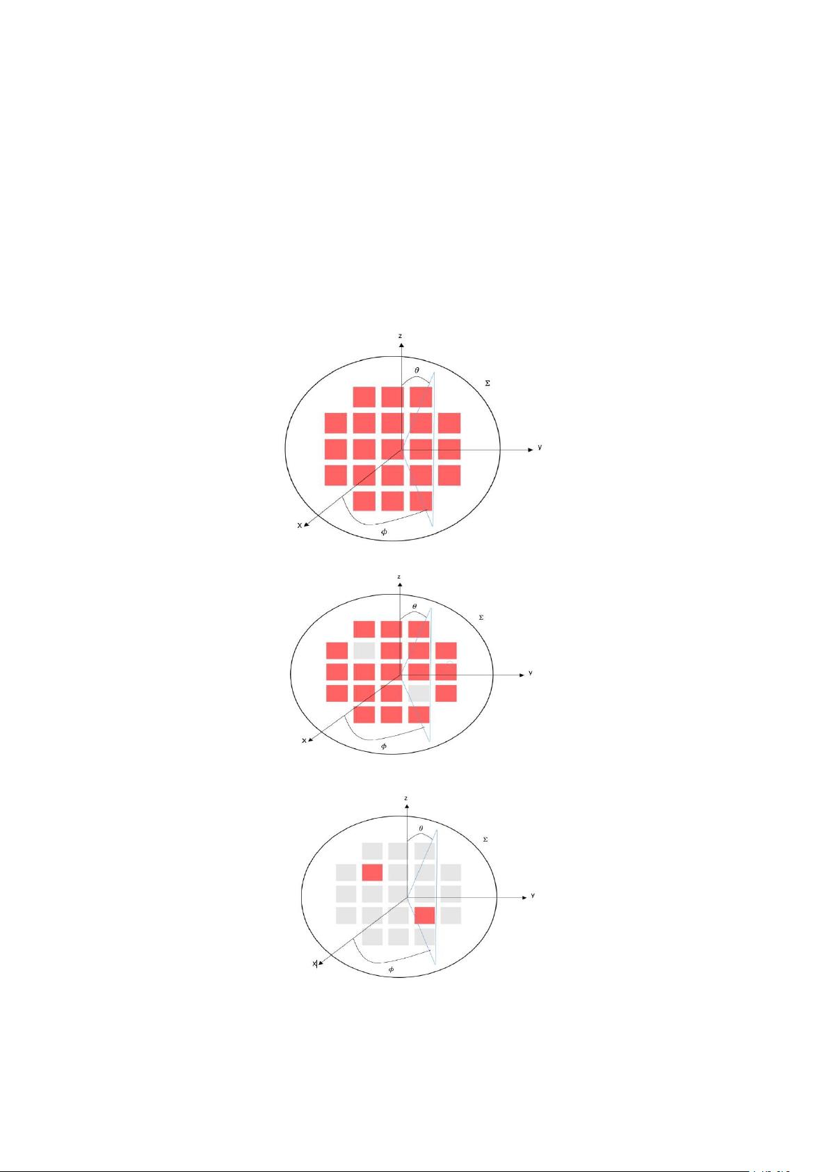
Figure 2. Antenna array: (a) reference antenna without failures; (b) antenna under test (AUT); (c)
differential antenna (DA). The number of failures is 2 within the total element number N = 21.
Figure 2.
Antenna array: (
a
) reference antenna without failures; (
b
) antenna under test (AUT);
(c) differential antenna (DA). The number of failures is 2 within the total element number N = 21.
剩余22页未读,继续阅读

qq_37788823
- 粉丝: 2
- 资源: 14
 我的内容管理
展开
我的内容管理
展开


最新资源
- 最优条件下三次B样条小波边缘检测算子研究
- 深入解析:wav文件格式结构
- JIRA系统配置指南:代理与SSL设置
- 入门必备:电阻电容识别全解析
- U盘制作启动盘:详细教程解决无光驱装系统难题
- Eclipse快捷键大全:提升开发效率的必备秘籍
- C++ Primer Plus中文版:深入学习C++编程必备
- Eclipse常用快捷键汇总与操作指南
- JavaScript作用域解析与面向对象基础
- 软通动力Java笔试题解析
- 自定义标签配置与使用指南
- Android Intent深度解析:组件通信与广播机制
- 增强MyEclipse代码提示功能设置教程
- x86下VMware环境中Openwrt编译与LuCI集成指南
- S3C2440A嵌入式终端电源管理系统设计探讨
- Intel DTCP-IP技术在数字家庭中的内容保护
资源上传下载、课程学习等过程中有任何疑问或建议,欢迎提出宝贵意见哦~我们会及时处理!
点击此处反馈


