By utilizing the gridding spatial partition approach, the contin-
uous spatial domain can be simply represented by the discrete grid
cells. Accordingly, the problem of trajectory pattern mining can be
reduced into a sequence pattern mining problem, so that many
conventional sequence pattern mining techniques can be applied
to this problem.
Although the grid-based approach can solve the spatial approx-
imation concern to a certain degree as mentioned above, it causes
the sharp boundary problem. That is, when some approximate tra-
jectory locations are close to the boundary of predetermined grid
cells, they will be most likely assigned to different cells by the
strict boundary constraints. Therefore, some potential meaningful
patterns will not be discovered due to this issue. In other words,
the approximate trajectory locations may span more than one grid
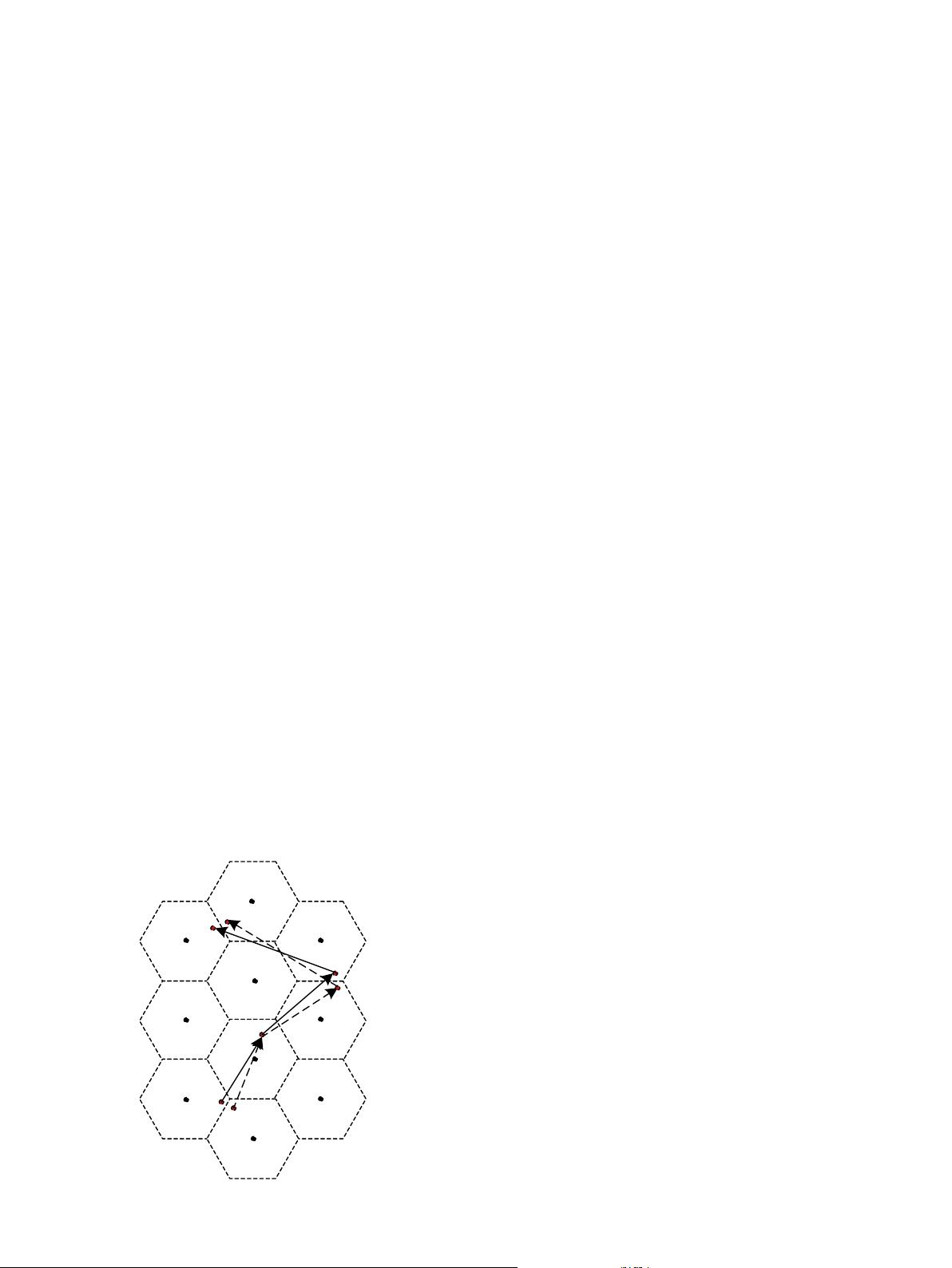
cell using the crisp gridding spatial partition approach. Considering
a scenario shown in Fig. 1, two similar and close trajectory in-
stances, Tr
1
={p
1
, p
2
, p
3
, p
4
} and Tr
2
¼fp
0
1
; p
0
2
; p
0
3
; p
0
4
g, are regarded
as two different moving behaviors s
7
? s
8
? s
3
? s
1
and
s
10
? s
8
? s
6
? s
2
in the crisp space partition way. However, it is
obvious that these two trajectories share the same moving pattern.
This example clearly suggests that the crisp grid space partition
method is sensitive to spatial noise. If mobile objects with similar
trajectory pattern do not exactly follow the same trajectories, the
implicit pattern cannot be detected.
However, in practice, we do not expect a mobile object to visit
exactly the same location at every time instant during each time
period. In addition, due to the limited energy supply of sensor de-
vice and location precision errors, the trajectory readings from
these devices always carry uncertain information. In that case, the
sharp boundary problem will deteriorate drastically with increas-
ing noise. Actually, the regular crisp space partition method can
be seen as a hard partition way with strict boundary constraints.
From Fig. 1, we can learn that the hard partition way is very likely
to cause the sharp boundary problem. Therefore, we consider divid-
ing the spatial plane via a flexible partition way to approximate
close trajectory locations and tackle the sharp boundary problem.
3.2. Problem definition
Definition 1. The time interval in a moving trajectory between any
two trajectory locations hx
i
, y
i
, t
i
i and hx
j
, y
j
, t
j
i is defined as
D
t = t
j
t
i
, where t
j
> t
i
. For example, the consecutive time intervals
of a moving trajectory Tr
2
={h p
1
,2i, hp
3
,5i, hp
7
,10i } are 3 and 5
respectively, and the transformed form of the moving trajectory
with time intervals is represented as p
1
!
3
p
3
!
5
P
7
.
Definition 2. A trajectory pattern in this work is defined as r
i
!
D
t
r
j
,
where r
i
and r
j
denote the spatial grid cell labels, and
D
t is a time
interval between these two cells. A pattern with k-length is called
k-pattern. Actually, a k-pattern is comprised of k grid cells and
(k 1) time intervals.
Definition 3. The space membership value is defined as the mem-
bership degree of the trajectory location hx
i
, y
i
i to the spatial grid
cell r
i
.
Actually, the space membership value is inversely proportional
to the relative distance between hx
i
, y
i
i and r
i
. By means of a mem-
bership function, the trajectory location hx
i
, y
i
i can be transformed
into the grid-labeled data hr
i
, m
i
i, where r
i
is the label of assigned
grid cell and m
i
denotes the corresponding membership value.
Note that the trajectory location hx
i
, y
i
i may be mapped into more
than one neighboring grid cell with membership values.
Definition 4. The number of partitioned spatial grid cells e is
defined as the desired space granularity to view the spatial data.
The larger the value e is, the finer the granularity of space is. On the
contrary, the smaller the number of the partitioned grid cells is, the
coarser the space granularity is.
However, selecting the value of e in data analysis is not trivial.
Too large granularity may damage the pattern semantics, while too
small granularity may result in a small number (or none in the
worst case) of patterns and high computation cost. In practice, e
can be determined based on domain knowledge.
Definition 5. In the vague space partition, the crisp zone radius r is
defined as the ratio of crisp zone area to the unit grid cell area.
Unlike the regular grid cell, the vague grid cell is comprised of a
crisp zone and an intermediate zone. Trajectory location distrib-
uted in the crisp zone is exclusively assigned to the grid cell con-
taining it with a constant membership value 1. But for the
intermediate zone, location situated in it may be assigned to more
than one neighboring cell.
Definition 6. A frequent trajectory pattern is that whose total
support in database is not less than the user-specified minimum
support threshold minsup.
Given a trajectory database D, a vague space partition member-
ship function and a minimum support threshold minsup, the objec-
tive of mining frequent trajectory pattern is to find the complete
set of the frequent patterns, i.e., all trajectory patterns r
i
!
D
t
i
r
j
.
4. Proposed method
4.1. Vague space partition method
In this subsection we will discuss how to partition the spatial
plane flexibly by vague way, and how to convert the original trajec-
tory dataset into transformed trajectory sequences.
Inspired by the rough set theory, we consider dividing the reg-
ular grid cell into a crisp zone and an intermediate zone. By this
way, we can build a novel grid cell, namely vague grid cell. Fig. 2
depicts three vague grid cells, s
1
, s
2
and s
3
, which are distributed
uniformly over the spatial plane. The part inside the circle of vague
grid cell is defined as the crisp zone, and the one outside the crisp
1
s
2
s
3
s
4
s
5
s
6
s
7
s
8
s
9
s
10
s
1
p
2
p
3
p
4
p
'
1
p
'
2
p
'
3
p
'
4
p
Fig. 1. Example of the sharp boundary problem.
102 L. Wang et al. / Knowledge-Based Systems 50 (2013) 100–111


