2
(a) (b) (c)
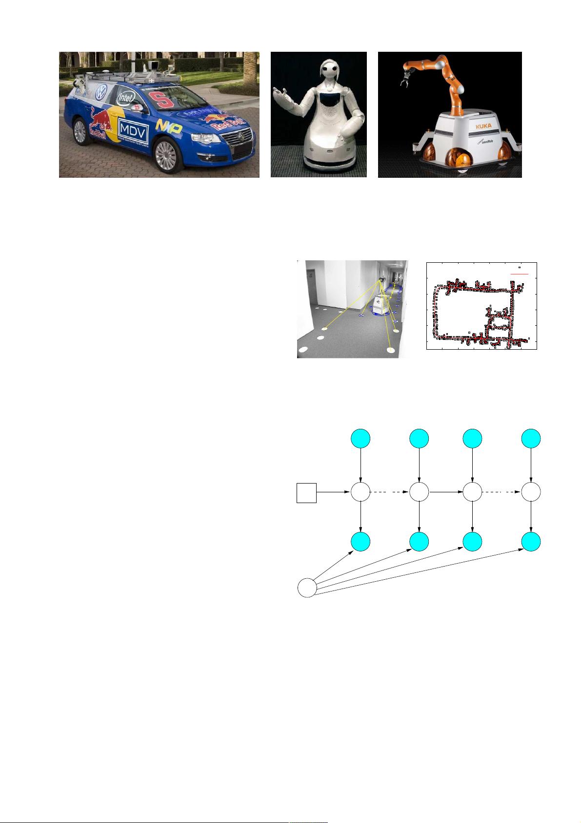
Fig. 1. Applications of SLAM technology. (a) An autonomous instrumented car developed at Stanford. This car can acquire maps by utilizing only its
on-board sensors. These maps can be subsequently used for autonomous navigation. (b) The museum guide robot TPR-Robina developed by Toyota (picture
courtesy of Toyota Motor Company). This robot acquires a new map every time the museum is reconfigured. (c) The KUKA Concept robot “Omnirob”, a
mobile manipulator designed autonomously navigate and operate in the environment with the sole use of its on-board sensors (picture courtesy of KUKA
Roboter GmbH).
variables x
1:T
= {x
1
, . . . , x
T
}. While moving, it acquires a
sequence of odometry measurements u
1:T
= {u
1
, . . . , u
T
}
and perceptions of the environment z
1:T
= {z
1
, . . . , z
T
}.
Solving the full SLAM problem consists of estimating the
posterior probability of the robot’s trajectory x
1:T
and the
map m of the environment given all the measurements plus
an initial position x
0
:
p(x
1:T
, m | z
1:T
, u
1:T
, x
0
). (1)
The initial position x
0
defines the position of the map and
can be chosen arbitrarily. For convenience of notation, in the
remainder of this document we will omit x
0
. The poses x
1:T
and the odometry u
1:T
are usually represented as 2D or 3D
transformations in SE(2) or in SE(3), while the map can be
represented in different ways. Maps can be parametrized as
a set of spatially located landmarks, by dense representations
like occupancy grids, surface maps, or by raw sensor measure-
ments. The choice of a particular map representation depends
on the sensors used, on the characteristics of the environment,
and on the estimation algorithm. Landmark maps [28], [22] are
often preferred in environments where locally distinguishable
features can be identified and especially when cameras are
used. In contrast, dense representations [33], [12], [9] are
usually used in conjunction with range sensors. Independently
of the type of the representation, the map is defined by the
measurements and the locations where these measurements
have been acquired [17], [18]. Figure 2 illustrates three typical
dense map representations for 3D and 2D: multilevel surface
maps, point clouds and occupancy grids. Figure 3 shows a
typical 2D landmark based map.
Estimating the posterior given in (1) involves operating in
high dimensional state spaces. This would not be tractable if
the SLAM problem would not have a well defined structure.
This structure arises from certain and commonly done assump-
tions, namely the static world assumption and the Markov
assumption. A convenient way to describe this structure is via
the dynamic Bayesian network (DBN) depicted in Figure 4.
A Bayesian network is a graphical model that describes a
stochastic process as a directed graph. The graph has one node
for each random variable in the process, and a directed edge (or
-20
-10
0
10
20
30
-50 -40 -30 -20 -10 0 10 20
landmarks
trajectory
Fig. 3. Landmark based maps acquired at the German Aerospace Center. In
this setup the landmarks consist in white circles painted on the ground that
are detected by the robot through vision, as shown in the left image. The right
image illustrates the trajectory of the robot and the estimated positions of the
landmarks. These images are courtesy of Udo Frese and Christoph Hertzberg.
x
0
x
1
x
t−1
x
t
x
T
u
1
u
t−1
u
t
u
T
z
1
z
t−1
z
t
z
T
m
Fig. 4. Dynamic Bayesian Network of the SLAM process.
arrow) between two nodes models a conditional dependence
between them.
In Figure 4, one can distinguish blue/gray nodes indicating
the observed variables (here z
1:T
and u
1:T
) and white nodes
which are the hidden variables. The hidden variables x
1:T
and m model the robot’s trajectory and the map of the
environment. The connectivity of the DBN follows a recurrent


