494 A. Larranaga et al. / Physics Letters B 743 (2015) 492–502
This equation cannot be solved for r
H
in a closed form, but,
by plotting f
(
r
)
one can determine numerically the existence of
horizon(s) and their radius by reading the intersections with the
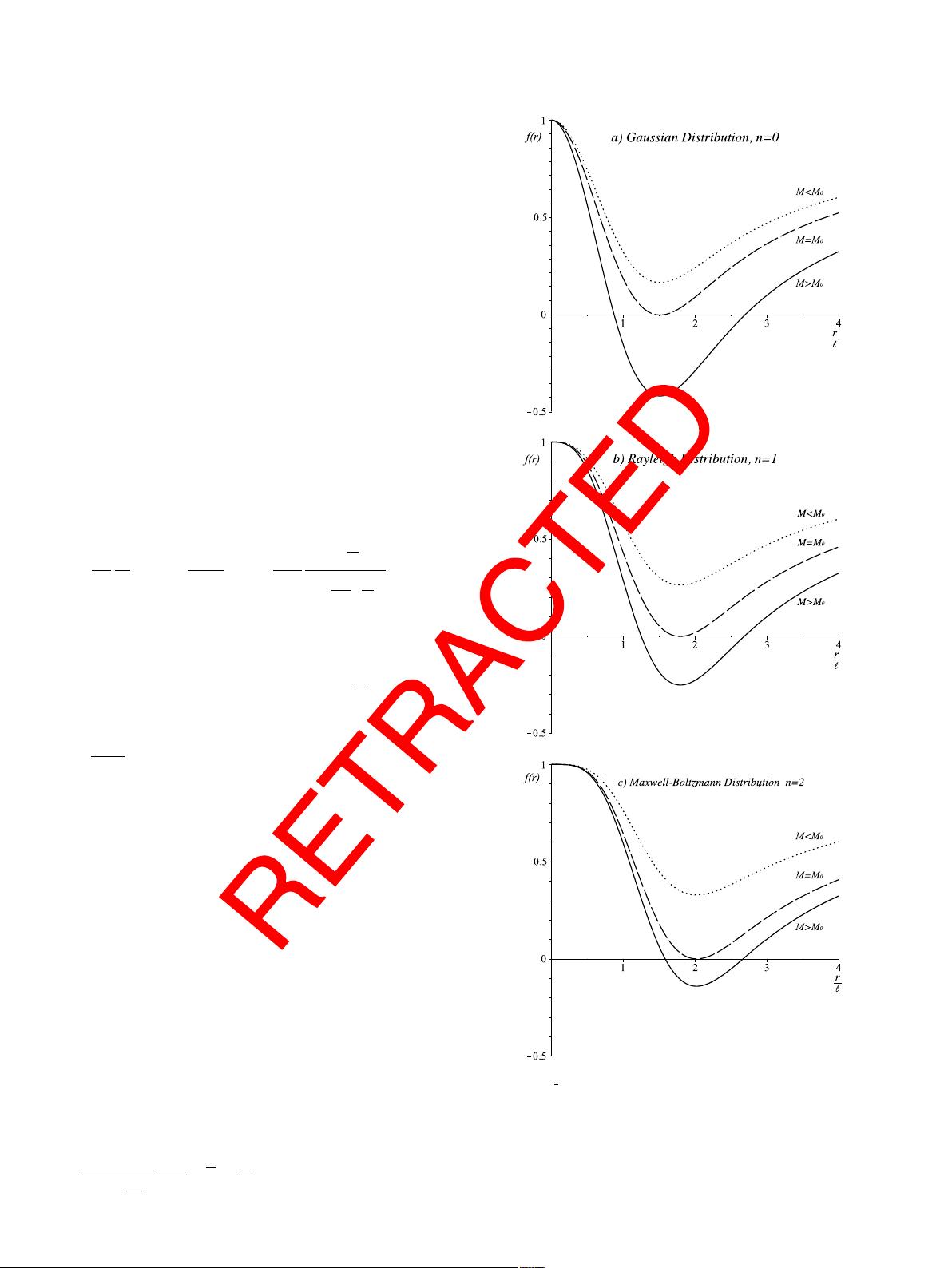
r-axis. From Fig. 1 is easy to note that the smeared mass distribu-
tion
introduces new behavior with respect to Schwarzschild black
hole. In fact, instead of a single event horizon, for each value of n
in
f
(
r
)
, there are three different possibilities:
1. two
distinct horizons for M > M
0
;
2. one
degenerate horizon in r
0
, corresponding to an extremal
black hole;
3. no
horizon for M < M
0
.
Therefore,
we conclude that there is no black hole if the orig-
inal
mass is less than the minimal mass M
0
which depends on
the value of the length and on the exponent n. Furthermore,
contrary to the usual Schwarzschild black hole, there can be two
horizons for large masses. It also can be seen that for M M
0
, the
inner
horizon shrinks to zero while the outer one approaches the
Schwarzschild horizon, located at r
S
= 2M.
2.1. Thermodynamics
The temperature associated with the black hole is given by
T =
1
4π
df
dr
r=r
H
=
1
4πr
H
⎡
⎢
⎢
⎣
1 −2
r
n+3
H
n+3
e
−
r
2
H
2
γ
n+3
2
,
r
2
H
2
⎤
⎥
⎥
⎦
,
(11)
where we have used the derivative of the lower incomplete gamma
function and Eq. (10) to write M in terms of r
H
. It is clear that the
second term inside the brackets is the correction arising from the
smeared distribution. For large black holes, i.e.,
r
2
H
2
1, Eq. (11)
recovers
the standard Hawking temperature for the Schwarzschild
black hole,
T
H
=
1
4πr
H
. (12)
In Fig. 2 we plot the temperature (11) as a function of r
H
and
we find that at the initial state of evaporation the black hole tem-
perature
increases while the horizon radius is decreasing. Here, the
interesting point is to investigate what happens as we reach the
final state of the process, i.e., when r
H
→ . As is well-known, in
the standard case the Hawking temperature T
H
diverges as M → 0,
or equivalently r
H
→ 0. However, in our solution the temperature
(11) deviates from the standard hyperbola (12) and instead of ex-
ploding,
it reaches a maximum value and then it quickly drops to
zero for r
H
=r
0
, leaving a frozen extremal black hole. In the region
r
H
< r
0
there is no black hole, because physically T cannot be neg-
ative.
As is easily observed, the Hawking paradox is circumvented
by the smeared mass distribution.
2.2. Curvature scalars
We approach the regularity problem of the solution by studying
the behavior of two curvature scalars, the Ricci scalar R = g
μν
R
μν
with R
μν
the Ricci tensor, and the Kretschmann invariant K =
R
μνρσ
R
μνρσ
with R
μνρσ
the Riemann tensor. For our black hole
solution, these invariants are
R =
M
2π
n+3
2
r
n
n+3
e
−
r
2
2
2
r
2
2
−
(
n + 4
)
(13)
Fig. 1. f
(
r
)
vs
r
, for various values of n. Intercepts on the horizontal axis give radii
of the event horizons. Panel a) shows the Gaussian distribution, n =0, panel b) cor-
responds
to the Rayleigh distribution, n = 1and panel c) is the Maxwell–Boltzmann
distribution, n = 2. In all cases the continuous line represents a black hole with two
horizons, M > M
0
, the dashed line corresponds to the extreme black hole with one
degenerate horizon, M = M
0
, and the dotted line shows a solution with no hori-
zons
M < M
0
. The specific value of M
0
depends on the value of the length and
on the exponent n.


