粒子滤波：视觉跟踪中的多模态动态追踪算法

需积分: 9 34 浏览量更新于2024-08-01 收藏 405KB PDF 举报

粒子滤波在视觉跟踪中的应用是解决密集视觉环境中复杂目标追踪难题的一种创新方法。相比于经典的卡尔曼滤波，它依赖于非线性建模和非高斯概率分布，这使得算法能够处理多模态的场景，即同时考虑多种可能的假设。本文（International Journal of Computer Vision, 1998）由Isard和Blake撰写，他们提出的Condensation算法利用了“因子采样”技术，这是一种先前在静态图像理解中的概念，通过生成随机样本集来表示可能的解释。 Condensation算法的核心思想是结合学习到的动态模型与视觉观测，实时地更新这个随机样本集合。这种方法特别适用于处理敏捷运动的目标，即使在具有大量视觉干扰（clutter）的环境中也能提供高度鲁棒的跟踪性能。虽然采用了随机过程的方法，但 Condensation 的设计目标是在接近实时的条件下运行，这在处理实时视觉任务时显得尤为重要。在论文中，作者详细探讨了在密集视觉杂乱中追踪曲线的问题，指出传统的基于高斯分布的卡尔曼滤波由于其单峰特性，在处理这种复杂的不确定性场景时显得力不从心。通过 Condensation，作者展示了如何通过动态模型的学习和迭代处理，有效地捕捉和预测目标的轨迹，克服了传统方法的局限性。这篇经典文章引入了一种新颖的粒子滤波方法，它不仅扩展了视觉跟踪的理论框架，而且在实际应用中展现了强大的性能和实用性，特别是在处理动态物体跟踪的挑战性问题上。这对于现代计算机视觉和机器人技术的发展产生了深远的影响。

Condensation—Conditional Density Propagation for Visual Tracking 9

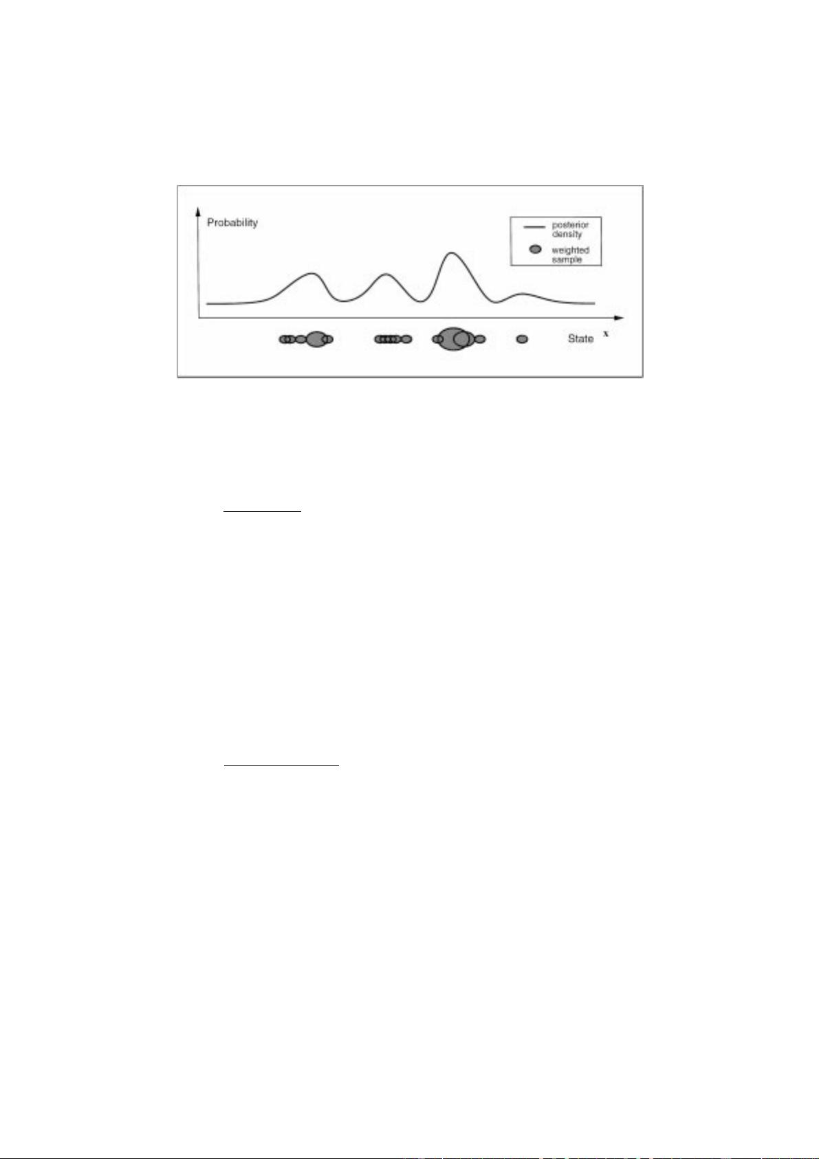
Figure 3. Factored sampling: a set of points s

(n)

, the centres of the blobs in the ﬁgure, is sampled randomly from a prior density p(x). Each

sample is assigned a weight π

(depicted by blob area) in proportion to the value of the observation density p(z |x = s

(n)

). The weighted

point-set then serves as a representation of the posterior density p(x |z), suitable for sampling. The one-dimensional case illustrated here extends

naturally to the practical case that the density is deﬁned over several position and shape variables.

n ∈{1,...,N}is chosen with probability π

, where

(n)

j=1

( j)

and

(x) = p(z |x),

the conditional observation density. The value x

= x

chosen in this fashion has a distribution which approx-

imates the posterior p(x |z) increasingly accurately as

N increases (Fig. 3).

Note that posterior mean properties E [g(x) |z] can

begenerateddirectlyfromthesamples{s

(n)

}byweight-

ing with p

(x) to give:

E[g(x) |z] ≈

n=1

(n)

n=1

(n)

. (7)

Forexample, themeancanbeestimatedusing g(x) = x

(illustrated in Fig. 4) and the variance using g(x) =

. In the case that p(x) is a spatial Gauss-Markov

process, Gibbs sampling from p(x) has been used

to generate the random variates {s

(1)

,...,s

(N)

}. Oth-

erwise, for low-dimensional parameterisations as in

this paper, standard, direct methods can be used for

Gaussians

(Press et al., 1988). Note that, in the case

that the density p(z |x) is normal, the mean obtained

by factored sampling is consistent with an estimate ob-

tained more conventionally, and efﬁciently, from linear

least squaresestimation. For multi-modal distributions

which cannot be approximated as normal, so that linear

estimators are unusable, estimates of mean x by fac-

tored sampling continue to apply.

4. The C

ONDENSATION Algorithm

The Condensation algorithm is based on factored

samplingbutextendedtoapplyiteratively to successive

images in a sequence. The same sampling strategy

has been developed elsewhere (Gordon, et al., 1993;

Kitagawa,1996), presentedasdevelopments ofMonte-

Carlo methods. Jump-diffusion tracking (Miller et al.,

1995) may also be related to the approach described

here.

Given that the process at each time-step is a self-

contained iteration of factored sampling, the out-

put of an iteration will be a weighted, time-stamped

sample-set, denoted {s

(n)

, n = 1,...,N}with weights

(n)

, representing approximately the conditional state-

density p(x

) at time t. How is this sample-set

obtained? Clearly, the process must begin with a prior

density and the effective prior for time-step t should

be p(x

t−1

). This prior is of course multi-modal in

general and no functional representation of it is avail-

able. It is derived from the sample set representation

{(s

(n)

t−1

,π

(n)

t−1

), n = 1,...,N} of p(x

t−1

), the

output from the previous time-step, to which predic-

tion (5) must then be applied.

The iterative process as applied to sample-sets, de-

picted in Fig. 5, mirrors the continuous diffusion pro-

cess in Fig. 2. At the top of the diagram, the out-

put from time-step t − 1 is the weighted sample-set

{(s

(n)

t−1

,π

(n)

t−1

), n = 1,...,N}. The aim is to maintain,

at successive time-steps, sample sets of ﬁxed size N,

剩余23页未读，继续阅读

niatzt

粉丝: 1
资源: 4

粒子滤波：视觉跟踪中的多模态动态追踪算法

PSO优化重采样粒子滤波：提升视觉跟踪性能

粒子滤波运动目标跟踪程序完整运行

基于粒子滤波的Matlab视觉跟踪技术

基于粒子群优化重采样的粒子滤波用于视觉跟踪

基于粒子滤波的视觉跟踪器的设计与实现

高斯噪声下粒子滤波用于目标跟踪的程序

利用多特征混沌粒子滤波的视觉目标跟踪方法

Muiltiple-Object-Tracking-master_目标跟踪_基于粒子滤波多目标跟踪实现_粒子滤波_

基于粒子滤波的物体跟踪

粒子滤波用于传感器目标跟踪，将观测值滤波估计出当前目标的位置

最新资源