基于稀疏表示的手机源验证:SCUTPHONE语音数据驱动
164 浏览量
更新于2024-08-26
收藏 1.25MB PDF 举报
本文探讨了在数字媒体取证领域中的一个重要新兴研究课题——源手机验证。传统的研究主要关注源记录设备的识别问题,而本文则着重填补了源手机验证这一领域的空白。作者提出了一种新颖的方法,即利用稀疏表示技术来增强手机验证系统的性能。
稀疏表示是一种在信号处理和机器学习中广泛应用的概念,它强调通过最小化信号在某种基下的系数数量来表达数据,这有助于捕捉数据的本质特征并提高模型的效率。在手机验证的背景下,稀疏表示有助于提取语音记录中与特定手机相关的独特模式。
作者提出了三种不同的稀疏表示方案:首先,使用示例词典,这种方法依赖于预先收集的特定手机的声音样本,能够识别个体手机的独特声学特性;其次,无监督学习词典,通过聚类或自组织映射等技术,自动学习设备间的差异,尽管可能牺牲部分判别能力;最后,监督学习词典,采用如支持向量机或深度神经网络等算法,结合大量标记数据,既保证了代表能力又提高了判别能力。
特别提到了基于MFCC(Mel频率倒谱系数)的高斯超向量(GSV),这是一种常用的技术,能有效地捕捉语音记录中固有的设备特性,用于构建和优化字典。MFCC是一种将音频信号转换为易于分析的特征表示,而高斯超向量则结合了统计特性,进一步提升了特征的区分度。
实验部分,作者使用了名为SCUTPHONE的数据集,该数据集包含15部不同手机的语音样本,验证了所提方法的有效性。通过对来自手机的三种语音记录进行评估,结果表明稀疏表示法在源手机验证任务上具有显著优势。此外,文章还深入探讨了示例词典中目标样本数量和无监督学习词典大小对验证性能的影响,这对于优化实际应用中的系统参数至关重要。
这篇研究论文不仅扩展了源记录设备验证的研究范围,而且引入了稀疏表示作为有效的工具,为手机身份验证提供了一种新的、基于统计学习的方法。这不仅在理论上推动了数字媒体取证领域的进展,也为实际应用提供了有价值的参考。
L. Zou et al. / Digital Signal Processing 62 (2017) 125–136 127
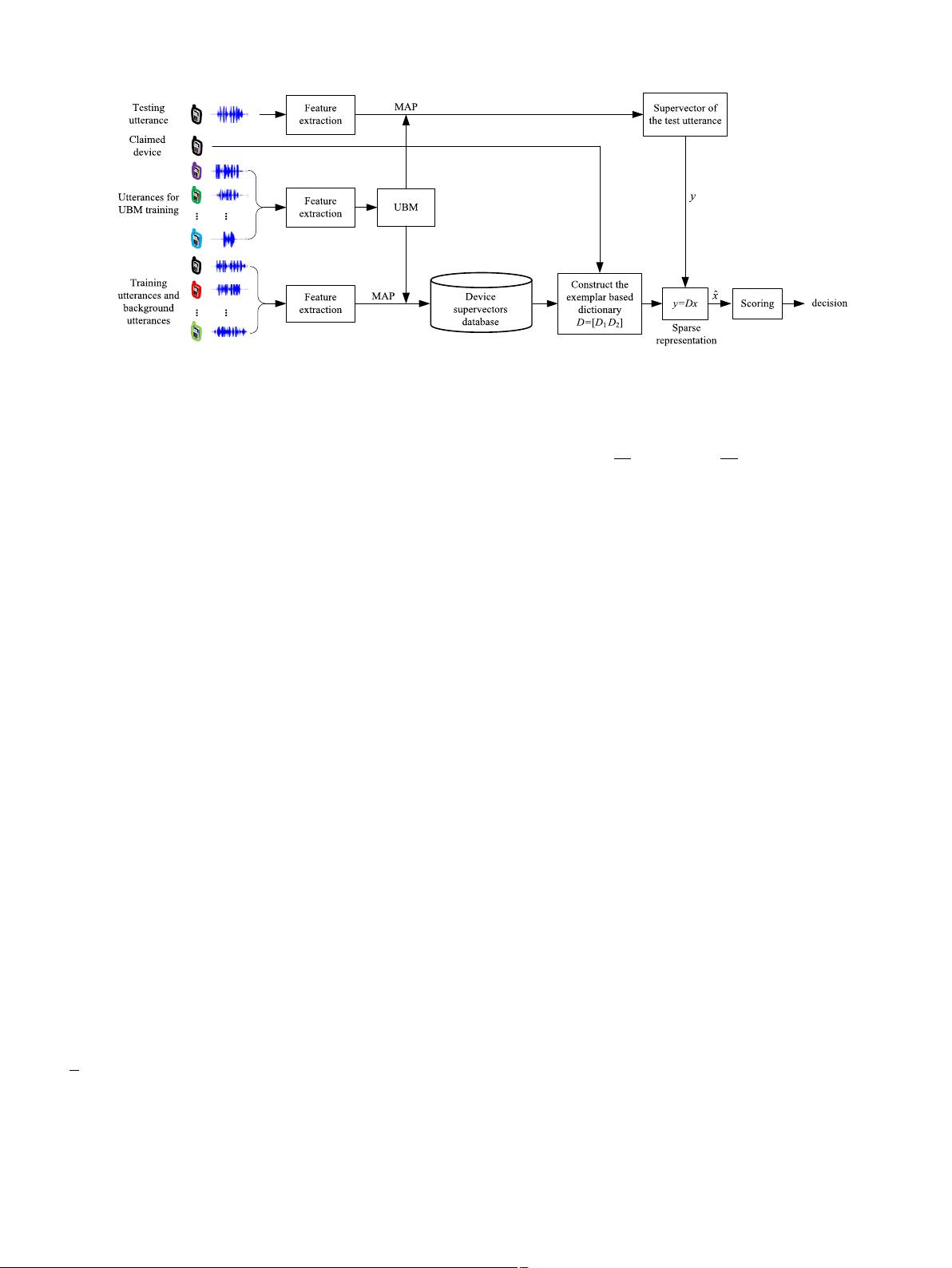
Fig. 1. Block diagram of source cell phone verification scheme based on sparse representation and exemplar dictionary.
show that the proposed scheme outperforms the exemplar dic-
tionary
based scheme, the unsupervised learned dictionary (here
K-SVD) based scheme and other two baseline methods. In addi-
tion,
we also analyze the influences of number of target examples
in exemplar dictionary and size of learned dictionary (by K-SVD)
on source cell phone verification performance.
The
rest of this paper is organized as follows. Section 2 de-
scribes
the method for extracting recording device intrinsic finger-
print.
Section 3 presents the sparse representation based source
cell phone verification schemes. Experimental setup and results
are provided in Section 4. Finally, conclusions and future work are
given in Section 5.
2. Recording device characterization
Over the last decade, various features were utilized to cap-
ture
the intrinsic characteristics of the recording devices. Gener-
ally
speaking, these features can be briefly grouped into three
categories: time domain, frequency domain and cepstral domain.
Specifically, mel-cepstral domain feature like MFCCs reported good
performance on source recording device recognition [26,27,44–46].
GSV, which is a high-dimensional vector (a.k.a. supervector) based
on low-dimensional feature vector (e.g., MFCCs), has been suc-
cessfully
applied to represent the intrinsic fingerprint of recording
device [26]. The signals in the speech recordings contain informa-
tion
not only related to recording device but also related to the
speech content such as speaker and linguistic information. It can
be deemed as the frequency response of the device contextual-
ized
by the speech content. GSV reduces the effects of the speech
content variability utilizing a statistical characterization of the fre-
quency
domain information of the contextualized signals.
The extraction procedure for GSV from a speech recording is
summarized as follows: Suppose that λ
UBM
={ω
i
, μ
i
,
i
}
M
i
=1
is a
diagonal covariance universal background model (UBM) with M
mixture
components, given a speech recording and the feature
vectors (here MFCCs) extracted from it, X ={x
t
}
T
t
=1
, the corre-
sponding
GMM is adapted from the UBM by adaptation of the
means through maximum a posteriori (MAP) [67,68]. More specif-
ically,
after computing the sufficient statistics for the weight and
mean parameters of mixture i as n
i
=
T
t
=1
P (i|x
t
) and E
i
(x) =
1
n
i
T
t
=1
P (i|x
t
)x
t
respectively, the ith adapted mean vector μ
i
is
computed as a weighted sum of the sufficient statistics for the
mean and the UBM mean: μ
i
= α
i
E
i
(x) + (1 − α
i
)μ
UBM
i
. Here,
α
i
is a data-dependent adaptation factor. It is defined as α
i
=
n
i
/(n
i
+ r) where r is a fixed relevance factor. Suppose that λ
a
=
{
ω
i
, μ
a
i
,
i
}
M
i
=1
and λ
b
={ω
i
, μ
b
i
,
i
}
M
i
=1
are the means adapted
GMMs corresponding to two speech recordings. The Kullback–
Leibler
(KL) divergence kernel is then defined as the corresponding
inner product of the GMM mean supervectors which is a concate-
nation
of the weighted GMM mean vectors [69]:
K (λ
a
,λ
b
) =
M
i=1
√
w
i
−1/2
i
μ
a
i
T
√
w
i
−1/2
i
μ
b
i
(1)
where M is the number of mixture components.
3. Cell phone verification by sparse representation
3.1. Scheme based on exemplar dictionary
We first present the exemplar dictionary based source cell
phone verification scheme. The corresponding block diagram is
shown in Fig. 1. During the verification process, for a claimed
device, N
1
target training examples (here GSV), represented as
{a
1i
}
N
1
i=1
, are placed together to construct D
1
=[a
11
, a
12
, ···, a
1N
1
] ∈
R
M×N
1
. At the same time, select N
2
non-target background exam-
ples,
represented as {a
2i
}
N
2
i=1
, from the background supervectors to
construct D
2
=[a
21
, a
22
, ···, a
2N
2
] ∈ R
M×N
2
and satisfy N
1
N
2
.
Thus, the exemplar dictionary is constructed by incorporating D
1
and D
2
as
D =[D
1
D
2
]
=[
a
11
, a
12
, ···,a
1N
1
, a
21
, a
22
, ···,a
2N
2
]∈R
M×N
(2)
where N = N
1
+ N
2
. Note that M < N should be satisfied for ob-
taining
a redundant and overcomplete dictionary. The atoms in
dictionary D are normalized to unit
2
-norm as in [55]. Then, given
a test vector y ∈ R
M
with unit
2
-norm and suppose that y can be
linearly represented with respect to D as
y = Dx =[D
1
D
2
]
x
1
x
2
(3)
where x is the coefficient vector. Fig. 2 shows an example of sparse
coefficient vectors for target and non-target trial. If y belongs to a
valid test, i.e., it comes from a speech recording recorded by the
claimed device, it will approximately lie in the linear span of the
columns of D
1
. Thus, the non-zero entries of coefficient vector x
associated
with D
1
(i.e., x
1
) will be large compared to the non-zero
entries of coefficient vector x associated with D
2
(i.e., x
2
) as shown
in Fig. 2(a). On the other hand, if y belongs to an invalid test, i.e.,
it comes from a speech recording, which is not recorded by the
claimed device, the coefficient vectors will be sparsely distributed
across D
1
and D
2
as shown in Fig. 2(b). The sparse solution to
(3) can be obtained by solving the following optimization problem
[66]:
剩余11页未读,继续阅读
点击了解资源详情
152 浏览量
点击了解资源详情
2021-03-08 上传
点击了解资源详情
点击了解资源详情
238 浏览量
点击了解资源详情
点击了解资源详情

weixin_38643269
- 粉丝: 2
 我的内容管理
展开
我的内容管理
展开


最新资源
- UML统一建模语言全方位指南
- VBS脚本基础教程:条件判断与逻辑运算
- C# 3.0 新特性详解:隐型变量、扩展方法与Lambda表达式
- VBS脚本入门教程6:FSO操作实践
- VBS入门教程5:FSO操作与文本文件创建
- VBS脚本入门教程4:使用WshShell对象控制应用程序
- VBS脚本基础教程:Windows命令与实战示例
- 源码追踪:名家经验与阅读策略
- 20世纪编程革命:OOP起源与发展
- 飞机订票系统实现与管理
- Windows主板BIOS设置详解与图解教程
- JAVA面试必备:基础知识点与异常处理
- 《代码大全2》:软件构建的艺术
- Hibernate入门指南:Java关系数据库持久化与配置详解
- Oracle SOA搭建指南
- C++批判:编程语言趋势与问题分析(第3版)
