CHAPTER 2 ■ MACHINE LEARNING FUNDAMENTALS
12
We now have all the details in place to discuss the core concept of generalization. The key question to ask
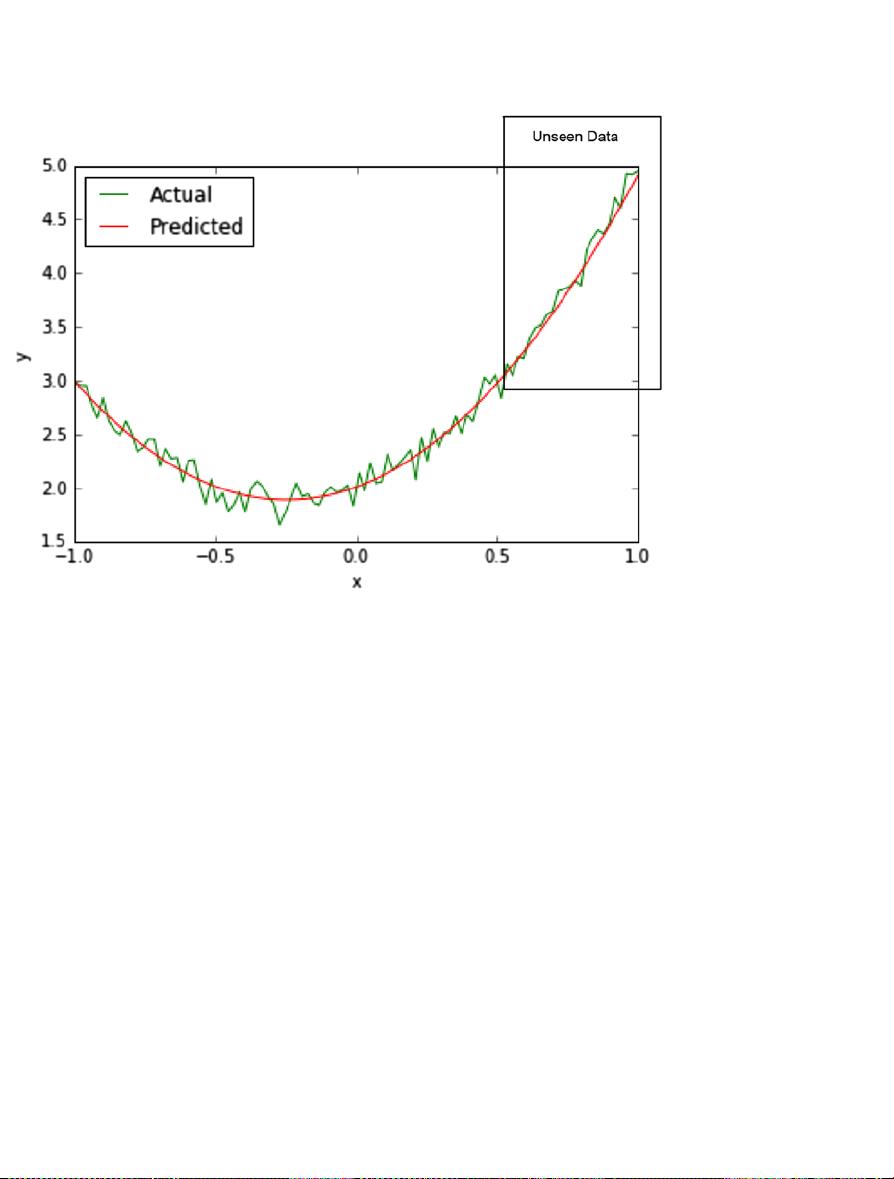
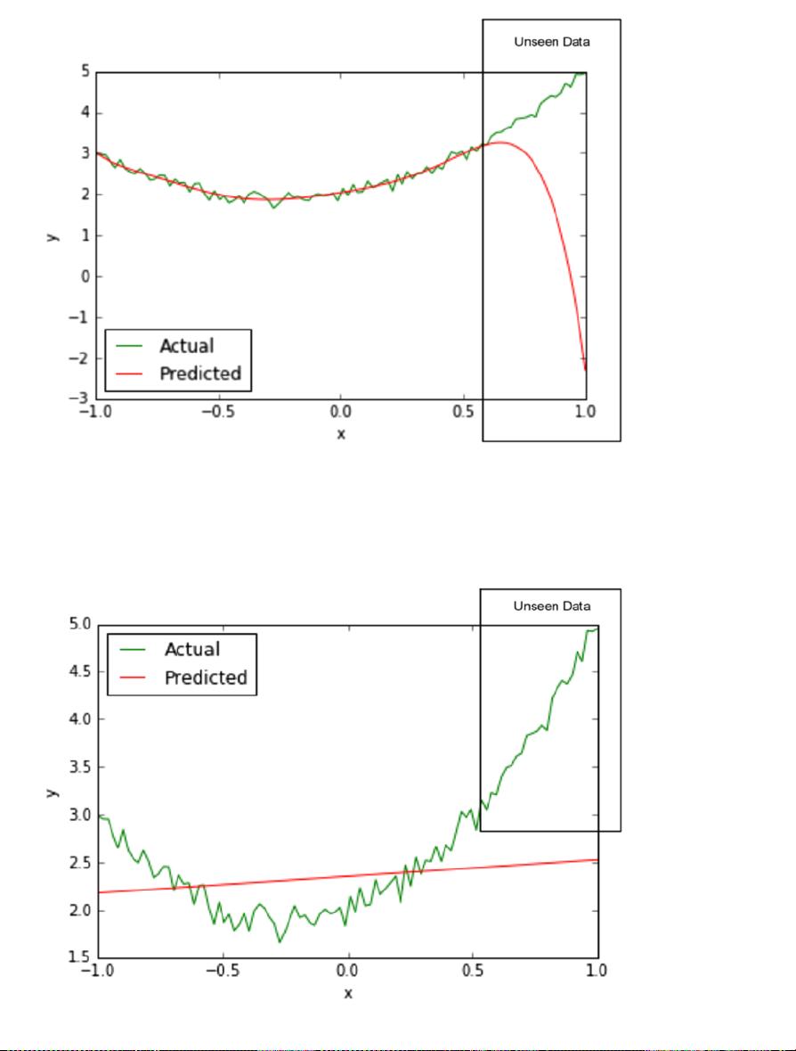
is which is the better model? The one with degree = 2 or the one with degree = 8 or the one with degree = 1?
Let us start by making a few observations about the three models. The model with degree = 1 performs
poorly on both the seen as well as unseen data as compared to the other two models. The model with
degree = 8 performs better on seen data as compared to the model with degree = 2. The model with
degree= 2 performs better than the model with degree = 8 on unseen data. Table2-1 visualizes this in table
form for easy interpretation.
Table 2-1. Comparing the performance of the 3 different models
Degree 1 2 8
Seen Data Worst Worst Better
Unseen Data Worst Better Worst
Let us now understand the important concept of model capacity, which corresponds to the degree of the
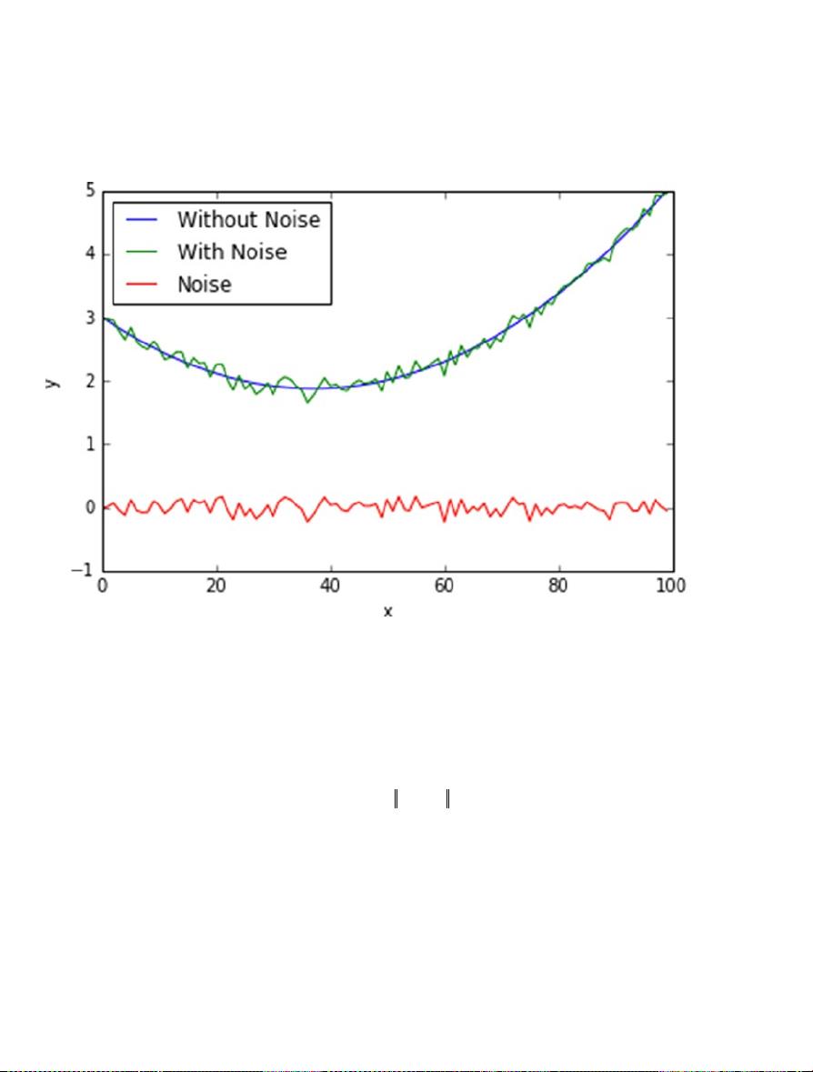
polynomial in this example. The data we generated was using a second order polynomial (degree = 2) with
some noise. Then, we tried to approximate the data using three models of degree: 1, 2, and 8, respectively.
The higher the degree, the more expressive is the model. That is, it can accommodate more variation. This
ability to accommodate variation corresponds to the notion of capacity. That is, we say that the model with
degree = 8 has a higher capacity that the model with degree = 2, which in turn has a higher capacity than
the model with degree = 1. Isn’t having higher capacity always a good thing? It turns out it is not, when we
consider that all real world datasets contain some noise and a higher capacity model will end up just fitting
the noise in addition to the signal in the data. This is why we observe that the model with degree = 2 does
better on the unseen data as compared to the model with degree = 8. In this example, we knew how the data
was generated (with a second order polynomial (degree = 2) with some noise); hence, this observation is quite
trivial. However, in the real world, we don’t know the underlying mechanism by which the data is generated.
This leads us to the fundamental challenge in machine learning, which is, does the model truly generalize?
And the only true test for that is the performance over unseen data.
In a sense the concept of capacity corresponds to the simplicity or parsimony of the model. A model
with high capacity can approximate more complex data. This is how many free variables/coefficients the
model has. In our example, the model with degree = 1 does not have capacity sufficient to approximate the
data and this is commonly referred to as under fitting. Correspondingly, the model with degree = 8 has extra
capacity and it over fits the data.
As a thought experiment, consider what would happen if we had a model with degree equal to 80. Given
that we had 80 data points as training data, we would have an 80-degree polynomial that would perfectly
approximate the data. This is the ultimate pathological case wherein there is no learning at all. The model
has 80 coefficients and can simply memorize the data. This is referred to as rote learning, the logical extreme
of overfitting. This is why the capacity of the model needs to be tuned with respect to the amount of training
data we have. If the dataset is small, we are better off training models with lower capacity.
Regularization
Building on the idea of model capacity, generalization, over fitting, and under fitting, let us now cover the
idea of regularization. The key idea here is to penalize complexity of the model. A regularized version of least
squares takes the form y =
x, where
is a vector such that Xy
b
-+
2
2
2
2
is minimized and λ is a
user-defined parameter that controls the complexity. Here, by introducing the term
lb
2
2
, we are penalizing
complex models. To see why this is the case, consider fitting a least square model using a polynomial of
degree 10, but the values in the vector
has 8 zeros; 2 are non-zeros. Against this, consider the case where


