基于LBP的动态纹理分析与面部表情识别方法
LBP人脸表情识别是一种基于LBP(Local Binary Pattern)技术在动态纹理分析领域的创新应用。论文由Guoying Zhao和Matti Pietikäinen(IEEE高级会员)共同提出,他们将传统的静态纹理分析扩展到了时间域,关注动态纹理(Dynamic Texture, DT)的描述和识别,这是一种结合了运动和外观特征的新型表示方式。
论文的核心贡献在于提出了一种新颖的基于VLBP(Volume Local Binary Pattern)的方法来处理动态纹理。VLBP是LBP的扩展,它不仅考虑像素点的局部纹理信息,还融合了空间邻域的运动特征,从而提高了对动态场景中面部表情等局部动态变化的敏感性。这种方法通过只关注三个互相垂直平面上的局部二值模式(LBP-TOP)的共出现情况,实现了算法的简化和易于扩展。
为了进一步增强处理能力,论文提出了一个基于块的策略。这种策略特别针对像面部表情这样需要同时考虑局部信息和位置关系的特定动态事件。这种方法确保了在处理面部表情识别时能够捕捉到局部细节和其在空间上的分布,从而提高识别精度。
实验部分展示了VLBP和LBP-TOP方法在两个动态纹理数据库,DynTex和MIT上卓越的表现。相比于传统方法,它们在识别动态纹理,特别是面部表情时,取得了明显的优势。这表明LBP人脸表情识别技术具有良好的鲁棒性和准确性,对于实际的人脸表情分析和识别应用具有很高的实用价值。通过学习这篇论文,读者可以了解到如何利用LBP技术提升动态场景下的人脸表情识别性能,并且理解如何将这一技术应用于实际的计算机视觉系统中。
the circularly symmetric neighborhood g
t;p
ðt ¼ t
c
L; t
c
;
t
c
þ L; p ¼ 0; ;P 1Þ, giving
V ¼ vðg
t
c
L;c
g
t
c
;c
;g
t
c
L;0
g
t
c
;c
; ;
g
t
c
L;P 1
g
t
c
;c
;g
t
c
;c
;g
t
c
;0
g
t
c
;c
; ;
g
t
c
;P 1
g
t
c
;c
;g
t
c
þL;0
g
t
c
;c
; ;
g
t
c
þL;P 1
g
t
c
;c
;g
t
c
þL;c
g
t
c
;c
Þ:
ð2Þ
Then, we assume that differences g
t;p
g
t
c
;c
are indepen-
dent of g
t
c
;c
, which allow us to factorize (2):
V vðg
t
c
;c
Þvðg
t
c
L;c
g
t
c
;c
;g
t
c
L;0
g
t
c
;c
; ;
g
t
c
L;P1
g
t
c
;c
;g
t
c
;0
g
t
c
;c
; ;g
t
c
;P1
g
t
c
;c
;
g
t
c
þL;0
g
t
c
;c
; ;g
t
c
þL;P1
g
t
c
;c
;g
t
c
þL;c
g
t
c
;c
Þ:
In practice, exact independence is not warranted; hence,
the factorized distribution is only an approximation of the
joint distribution. However, we are willing to accept a
possible small loss of information as it allows us to achieve
invariance with respect to shifts in gray scale. Thus, similar to
LBP in ordinary texture analysis [6], the distribution vðg
t
c
;c
Þ
describes the overall luminance of the image, which is
unrelated to the local image texture and, consequently, does
not provide useful information for DT analysis. Hence, much
of the information in the original joint gray-level distribution
(1) is conveyed by the joint difference distribution:
V
1
¼ v ðg
t
c
L;c
g
t
c
;c
;g
t
c
L;0
g
t
c
;c
; ;
g
t
c
L;P1
g
t
c
;c
;g
t
c
;0
g
t
c
;c
; ;g
t
c
;P1
g
t
c
;c
;
g
t
c
þL;0
g
t
c
;c
; ;g
t
c
þL;P1
g
t
c
;c
;g
t
c
þL;c
g
t
c
;c
Þ:
This is a highly discriminative texture operator. It
records the occurrences of various patterns in the neighbor-
hood of each pixel in a ð2ðP þ 1ÞþP ¼ 3P þ 2Þ-dimen-
sional histogram.
We achieve invariance with respect to the scaling of the
gray scale by considering simply the signs of the differences
instead of their exact values:
V
2
¼ v
sðg
t
c
L;c
g
t
c
;c
Þ;sðg
t
c
L;0
g
t
c
;c
Þ; ;
sðg
t
c
L;P1
g
t
c
;c
Þ;sðg
t
c
;0
g
t
c
;c
Þ; ;
sðg
t
c
;P1
g
t
c
;c
Þ;sðg
t
c
þL;0
g
t
c
;c
Þ; ;
sðg
t
c
þL;P1
g
t
c
;c
Þ;sðg
t
c
þL;c
g
t
c
;c
Þ
;
ð3Þ
where sðxÞ¼
1;x 0
0;x< 0
.
To simplify the expression of V
2
, we use V
2
¼ vðv
0
; ;
v
q
; ;v
3Pþ1
Þ, and q corresponds to the index of values in
V
2
orderly. By assigning a binomial factor 2
q
for each
sign sðg
t;p
g
t
c
;c
Þ, we transform (3) into a unique V LBP
L;P;R
number that characterizes the spatial structure of the local
volume DT:
V LBP
L;P;R
¼
X
3Pþ1
q¼0
v
q
2
q
: ð4Þ
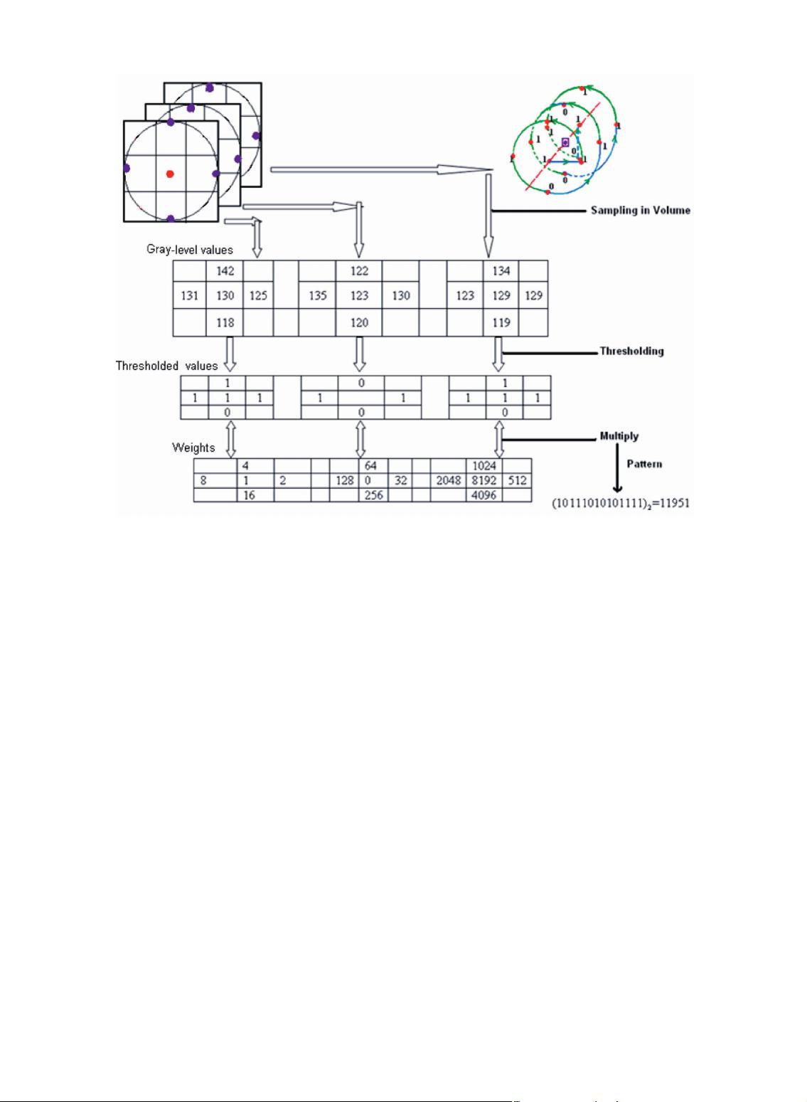
Fig. 1 shows the whole computing procedure for
V LBP
1;4;1
. We begin by sampling neighboring points in
the volume and then thresholding every point in the
neighborhood with the value of the center pixel to get a
binary valu e. Finally, we produce the VLBP code by
ZHAO AND PIETIKA
¨
INEN: DYNAMIC TEXTURE RECOGNITION USING LOCAL BINARY PATTERNS WITH AN APPLICATION TO FACIAL... 917
Fig. 1. Procedure of V LBP
1;4;1
.
下载后可阅读完整内容,剩余13页未读,立即下载
1513 浏览量
1069 浏览量
157 浏览量
2024-06-20 上传
2023-11-27 上传
2013-12-18 上传
2024-11-29 上传
2024-05-17 上传

youtubeIII
- 粉丝: 0
 我的内容管理
展开
我的内容管理
展开


最新资源
- C#与DevExpress控件开发软件教程
- 点状进度条dotted-progress-bar的Android实现与自调指南
- J2EE框架下的个人博客系统毕业设计
- 解决ECShop与jQuery冲突的兼容模式方案
- 2012版通达信公式函数使用详解与示例
- MIDI控制新体验:vi风格的MIDI连续控制器
- 51单片机应用设计与仿真教程
- Android超牛进度条组件使用与效果展示
- MATLAB中文帮助:实用操作指南
- 全面的TCP/UDP Socket调试解决方案
- Android手机游戏开发实践与市场分析
- 蜗牛进度条实现方法与seekbar应用示例
- 基于SQL与VB的医院管理系统设计与实现
- Snapshot:链下多管治理解决方案的探索与实践
- 操作系统进程管理与死锁检测技术解析
- 黑色红色调网站建设自助建站管理系统介绍