transformer
decoder
backbone
pixel
decoder
𝑁 queries
image features ℱ
per-pixel embeddings
MLP
𝑁 class predictions
𝑁 mask embeddings
𝑁 mask predictions
semantic segmentation
inference only
semantic
segmentation
classification loss
binary mask loss
𝐶
ℰ
×𝐻×𝑊
𝐶
ℰ
×𝑁
𝑁×𝐻×𝑊
𝑁×(𝐾 + 1)
𝐾×𝐻×𝑊
pixel-level module
segmentation moduletransformer module
drop ∅
𝒬
ℰ
"#$%&
ℰ
'()*
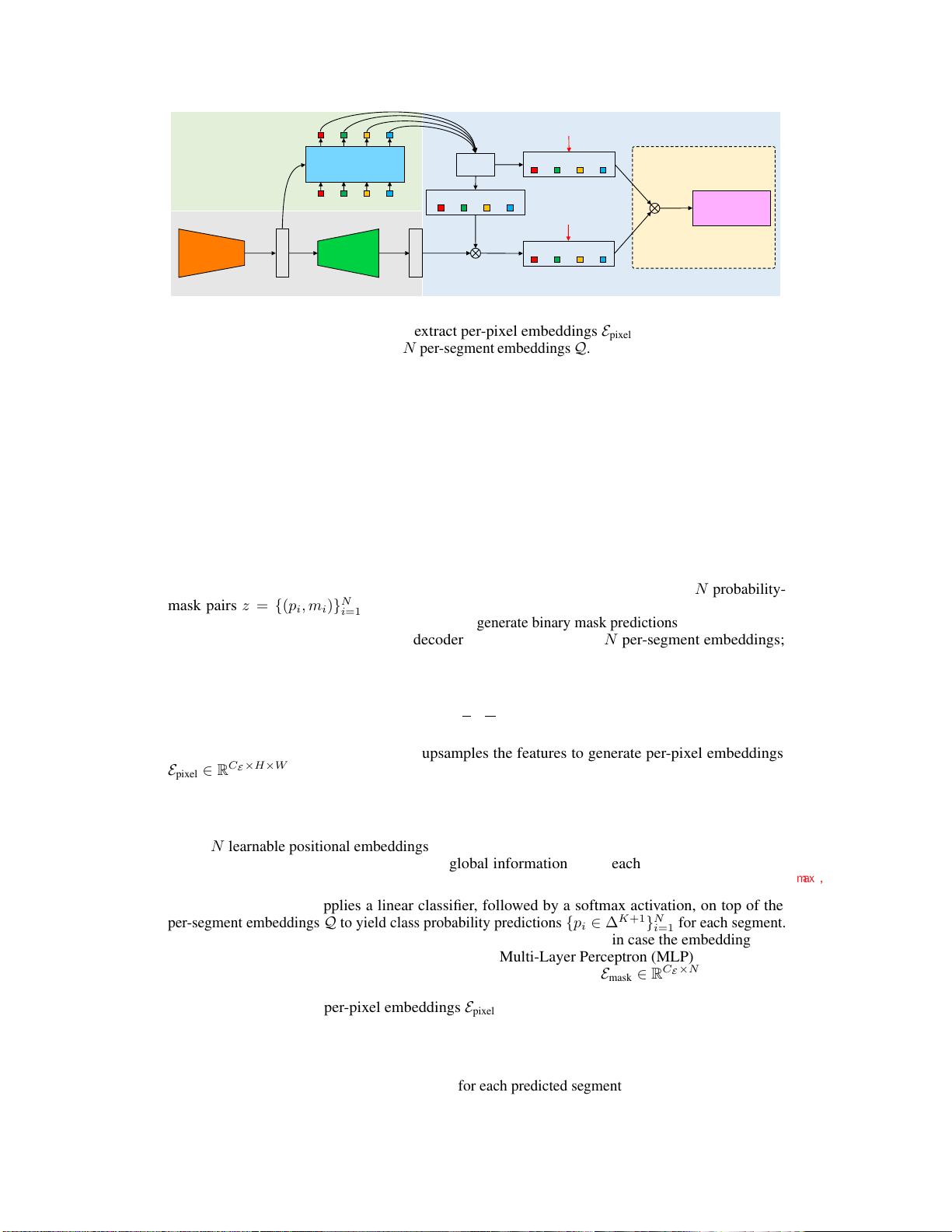
Figure 2:
MaskFormer overview.
We use a backbone to extract image features
F
. A pixel decoder
gradually upsamples image features to extract per-pixel embeddings
E
pixel
. A transformer decoder
attends to image features and produces
N
per-segment embeddings
Q
. The embeddings independently
generate
N
class predictions with
N
corresponding mask embeddings
E
mask
. Then, the model predicts
N
possibly overlapping binary mask predictions via a dot product between pixel embeddings
E
pixel
and mask embeddings
E
mask
followed by a sigmoid activation. For semantic segmentation task we
can get the final prediction by combining
N
binary masks with their class predictions using a simple
matrix multiplication (see Section 3.4). Note, the dimensions for multiplication
N
are shown in gray.
Note, that most existing mask classification models use auxiliary losses (e.g., a bounding box
loss [
21
,
4
] or an instance discrimination loss [
42
]) in addition to
L
mask-cls
. In the next section we
present a simple mask classification model that allows end-to-end training with L
mask-cls
alone.
3.3 MaskFormer
We now introduce MaskFormer, the new mask classification model, which computes
N
probability-
mask pairs
z = {(p
i
, m
i
)}
N
i=1
. The model contains three modules (see Fig. 2): 1) a pixel-level
module that extracts per-pixel embeddings used to generate binary mask predictions; 2) a transformer
module, where a stack of Transformer decoder layers [
41
] computes
N
per-segment embeddings;
and 3) a segmentation module, which generates predictions
{(p
i
, m
i
)}
N
i=1
from these embeddings.
During inference, discussed in Sec. 3.4, p
i
and m
i
are assembled into the final prediction.
Pixel-level module
takes an image of size
H × W
as input. A backbone generates a (typically)
low-resolution image feature map
F ∈ R
C
F
×
H
S
×
W
S
, where
C
F
is the number of channels and
S
is the stride of the feature map (
C
F
depends on the specific backbone and we use
S = 32
in this
work). Then, a pixel decoder gradually upsamples the features to generate per-pixel embeddings
E
pixel
∈ R
C
E
×H×W
, where
C
E
is the embedding dimension. Note, that any per-pixel classification-
based segmentation model fits the pixel-level module design including recent Transformer-based
models [37, 53, 29]. MaskFormer seamlessly converts such a model to mask classification.
Transformer module
uses the standard Transformer decoder [
41
] to compute from image features
F
and
N
learnable positional embeddings (i.e., queries) its output, i.e.,
N
per-segment embeddings
Q ∈ R
C
Q
×N
of dimension
C
Q
that encode global information about each segment MaskFormer
predicts. Similarly to [4], the decoder yields all predictions in parallel.
Segmentation module
applies a linear classifier, followed by a softmax activation, on top of the
per-segment embeddings
Q
to yield class probability predictions
{p
i
∈ ∆
K+1
}
N
i=1
for each segment.
Note, that the classifier predicts an additional “no object” category (
∅
) in case the embedding does
not correspond to any region. For mask prediction, a Multi-Layer Perceptron (MLP) with 2 hidden
layers converts the per-segment embeddings
Q
to
N
mask embeddings
E
mask
∈ R
C
E
×N
of dimension
C
E
. Finally, we obtain each binary mask prediction
m
i
∈ [0, 1]
H×W
via a dot product between the
i
th
mask embedding and per-pixel embeddings
E
pixel
computed by the pixel-level module. The dot
product is followed by a sigmoid activation, i.e., m
i
[h, w] = sigmoid(E
mask
[:, i]
T
· E
pixel
[:, h, w]).
Note, we empirically find it is beneficial to not enforce mask predictions to be mutually exclusive to
each other by using a softmax activation. During training, the
L
mask-cls
loss combines a cross entropy
classification loss and a binary mask loss
L
mask
for each predicted segment. For simplicity we use the
same
L
mask
as DETR [
4
], i.e., a linear combination of a focal loss [
27
] and a dice loss [
33
] multiplied
by hyper-parameters λ
focal
and λ
dice
respectively.
4
集合
upsamping
downsample
C H/S W/S
无缝的
这个是在channel上×的
,所以结果没有channel
了,其实可以视为通道
融合,和应用1*1卷积一
样
互斥
在某些情况下,对于预测的掩码(mask
)进行互斥约束(mutually exclusive
)并不总是有益的,因此在模型中使用
softmax 激活函数来实现互斥并不是必
须的。
使用 softmax 激活函数将掩码预测转换为概率分布,强制使每
个像素的预测值在所有类别上归一化,并且相互之间互斥。这
意味一个只能属于一个类别
首先一共分成了N个seg,这N个seg就当作vit中的patch进行处理了
重叠
输入的是 feature query进decoder
output:Q
Q是可以视为一个
整合了所有seg的
输出
Cq可以是一个
Segflatten出来
的维度(768)
N是Seg数,可以
patch中的一个
patch,也可以视
为query数
对每个向量(seg)做softmax,
预测自己属于哪一类
linear
N*Cq
linear
这一段的关键是,把Q当作decoder
出来的结果,每一行当作一个样本
的特征。就像做卷积的操作一样,
现在是提取完的feature_map。就
可以用linear做最后的收尾工作了


