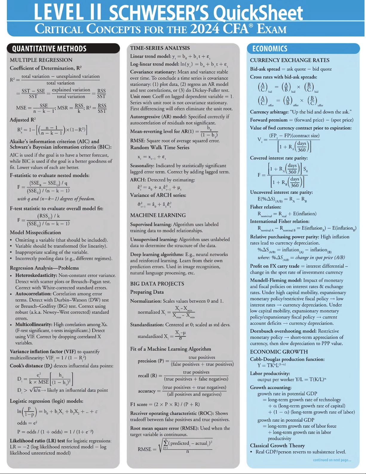
l Critical C oncepts for the 2024 CFA® Exam
QUANTITATIVE METHODS
MULTIPLE REGRESSION
Coefficient of Determination, R2
total variation — unexplained variation
R2 =
total variation
SST — SSE explained variation
SST total variation
RSS
SST
MSE =
SSE
-------------
• MSR = RSS- R2 = RSS
n-k-1’ k ’ SST
Adjusted R2
R2= 1 -
te^r)x(]-R2)
Akaikes information criterion (AIC) and
Schwarz s Bayesian information criteria (BIC):
AIC is used if the goal is to have a better forecast,
while BIC is used if the goal is a better goodness of
fit. Lower values of each are better.
F-statistic to evaluate nested models:
F =
(SSE
r - SSE„) / q
(SSEJ/fn-k- 1)
with q and (n—k—1) degrees o f freedom.
F-test statistic to evaluate overall model fit:
r (RSSu)/k
(SSEa) / (n — k — 1)
Model Misspecification
• Omitting a variable (that should be included).
• Variable should be transformed (for linearity).
• Inappropriate scaling of the variable.
• Incorrectly pooling data (e.g., different regimes).
Regression Analysis—Problems
• Heteroskedasticity: Non-constant error variance.
Detect with scatter plots or Breusch-Pagan test.
Correct with White-corrected standard errors.
• Autocorrelation: Correlation among error
terms. Detect with Durbin-Watson (DW) test
or Breusch-Godfrey (BG) test. Correct using
robust (a.k.a. Newey—West corrected) standard
errors.
• Multicollinearity: High correlation among Xs.
(F-test significant, t-tests insignificant.) Detect
using VIF. Correct by dropping correlated X
variables.
Variance inflation factor (VIF) to quantify
multicollinearity: VIF. = 1/(1 — R.2)
Cook’s distance (D.) detects influential data points:
D =
e2
i
r h..
11
k
x MSE
(i - h..)2
L ir
D. > v k / n —> likely an influential data point
Logistic regression (logit) models:
In
- b0 + blXl + b2X2 + " +
odds = e^
P = odds / (1 + odds) = 1 / ( 1 + e- y)
Likelihood ratio (LR) test for logistic regressions:
LR = — 2 (log likelihood restricted model — log
likelihood unrestricted model)
TIME-SERIES ANALYSIS
Linear trend model: y = b„ + b, t + e
J t 0 I t
Log-linear trend model: ln(y ) = b(i + b t t + £
Covariance stationary: Mean and variance stable
over time. To conclude a time series is covariance
stationary: (1) plot data, (2) regress an AR model
and test correlations, or (3) do Dickey-Fuller test.
Unit root: Coeff on lagged dependent variable = 1,
Series with unit root is not covariance stationary.
First differencing will often eliminate the unit root.
Autoregressive (AR) model: Specified correctly if
autocorrelation of residuals not significant.
Mean-reverting level for AR( 1) =
o
(1 - b , )
RMSE: Square root of average squared error.
Random Walk Time Series
xt = Xt-1 + c
Seasonality: Indicated by statistically significant
lagged error term. Correct by adding lagged term.
ARCH: Detected by estimating:
g? = ao + ai g?-i + H
Variance of ARCH series:
+i=ao + a,e.
MACHINE LEARNING
Supervised learning: Algorithm uses labeled
training data to model relationships.
Unsupervised learning: Algorithm uses unlabeled
data to determine the structure of the data.
Deep learning algorithms: E.g., neural networks
and reinforced learning. Learn from their own
prediction errors. Used in image recognition,
natural language processing, etc.
BIG DATA PROJECTS
Preparing Data
Normalization: Scales values between 0 and 1.
X -X .
normalized X. =
X - X
max min
Standardization: Centered at 0; scaled as std devs.
standardized X. =
a
Fit of a Machine Learning Algorithm
precision (P) =
recall (R) =
true positives
(false positives + true positives)
true positives
accuracy =
(true positives + false negatives)
(true positives + true negatives)
(all positives and negatives)
Fl score = (2
x P x R) / (P + R)
Receiver operating characteristic (ROC): Shows
tradeoff between false positives and true positives.
Root mean square error (RMSE): Used when the
target variable is continuous.
n
2 ( predicted. - actual.)
RMSE = " i=1
n
CURRENCY EXCHANGE RATES
Bid-ask spread = ask quote — bid quote
Cross rates with bid-ask spreads:
$L - (*
bid
x
bid x ^ ' bid
A
C
offer
4) X ( B
D 7 offer V ^ ' offer
Currency arbitrage: “Up the bid and down the ask.”
Forward premium = (forward price) — (spot price)
Value of fwd currency contract prior to expiration:
(FP — FP)(contract size)
V =
1 + R
days
360
Covered interest rate parity:
days
F =
1 + R
360
o
1 + R
B
days
360
Uncovered interest rate parity:
E(% A SW , = Ra - Rb
Fisher relation:
R . = R . + E(inflation)
nominal real
International Fisher relation:
R . .. — R . | = E(inflation,) — E(inflation„)
nominal A nominal d x A' v d '
Relative purchasing power parity: High inflation
rates lead to currency depreciation.
%AS,.m, = inflatio n .. . — inflation,-,
(A/B) (A) (B)
where: %AS(a/B) = change in spot price (A/B)
Profit on FX carry trade = interest differential -
change in the spot rate of investment currency
Mundell-Fleming model: Impact of monetary
and fiscal policies on interest rates & exchange
rates. Under high capital mobility, expansionary
monetary policy/restrictive fiscal policy —> low
interest rates —» currency depreciation. Under
low capital mobility, expansionary monetary
policy/expansionary fiscal policy —> current
account deficits —*• currency depreciation.
Dornbusch overshooting model: Restrictive
monetary policy —» short-term appreciation of
currency, then slow depreciation to PPP value.
ECONOMIC GROWTH
Cobb-Douglas production function:
Y = TKaL(1_ot)
Labor productivity:
output per worker Y/L = T(K/L)a
Growth accounting:
growth rate in potential GDP
= long-term growth rate of technology
+ ot (long-term growth rate of capital)
+ (1 — a) (long-term growth rate of labor)
growth rate in potential GDP
= long-term growth rate of labor force
+ long-term growth rate in labor
productivity
Classical Growth Theory
• Real GDP/person reverts to subsistence level.
continued on next page...


