霍夫变换新应用：通用方法检测任意形状

4星 · 超过85%的资源需积分: 10 55 浏览量更新于2024-09-23 1 收藏 838KB PDF 举报

本文是一篇深入探讨霍夫变换的经典论文，题目为《GENERALIZING THE HOUGH TRANSFORM TO DETECT ARBITRARY SHAPES》。作者D.H. BALLARD是计算机科学领域的专家，他在罗切斯特大学的研究表明，霍夫变换是一种强大的工具，最初主要用于检测二值图像中的曲线，无论是解析曲线（如直线、圆和抛物线）(1, 2, 3, 14, 15, 16)，还是非解析曲线。最初的霍夫变换方法不仅限于二值边缘检测，而是扩展到了灰度级图像中的一些解析曲线识别。特别地，它在检测线条（如边缘检测，应用广泛于诸如边缘检测算法、图像分割和机器视觉等领域，例如用于道路跟踪、指纹分析等应用中，见文献7, 8, 9）方面取得了显著成就。然而，本文的主要贡献在于进一步将霍夫变换的原理扩展到非解析形状的边界检测。作者提出了一种方法，将图像空间中的任意非解析形状边界映射到霍夫变换空间，这使得霍夫变换不再局限于特定类型的曲线，而是能够处理更复杂的形状。这种通用化的霍夫变换不仅增加了其在图像处理中的实用性，也为形状识别和特征提取提供了新的可能性。通过这篇文章，读者可以了解到如何利用霍夫变换的理论基础，对图像中的复杂形状进行有效分析，突破了早期方法的局限性，并为后续的研究者和实践者提供了处理非结构化形状检测的新思路。此外，文章可能还涵盖了霍夫变换的具体实现步骤、性能评估以及可能存在的挑战和改进方向，对于理解和应用霍夫变换在实际问题中的应用场景具有很高的参考价值。

Generalizing the Hough transform to detect arbitrary shapes 113

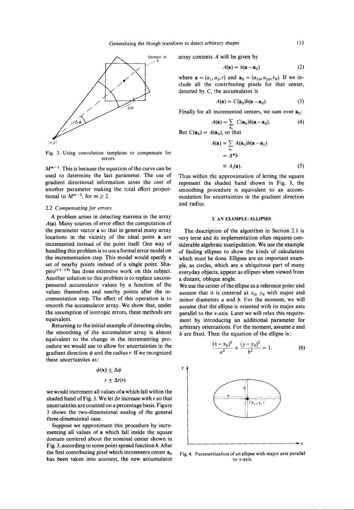
Oornoin of

(x,y)

Fig. 3. Using convolution templates to compensate for

errors.

M"- 1. This is because the equation of the curve can be

used to determine the last parameter. The use of

gradient directional information saves the cost of

another parameter making the total effort propor-

tional to M"-2, for m >_ 2.

2.2

Compensating for errors

A problem arises in detecting maxima in the array

A(a). Many sources of error effect the computation of

the parameter vector a so that in general many array

locations in the vicinity of the ideal point a are

incremented instead of the point itself. One way of

handling this problem is to use a formal error model on

the incrementation step. This model would specify a

set of nearby points instead of a single point. Sha-

piro tls-ls) has done extensive work on this subject.

Another solution to this problem is to replace uncom-

pensated accumulator values by a function of the

values themselves and nearby points after the in-

crementation step. The effect of this operation is to

smooth the accumulator array. We show that, under

the assumption of isotropic errors, these methods are

equivalent.

Returning to the initial example of detecting circles,

the smoothing of the accumulator array is almost

equivalent to the change in the incrementing pro-

cedure we would use to allow for uncertainties in the

gradient direction q~ and the radius r. If we recognized

these uncertainties as:

4~(x) + A~

r +_ Ar(r)

we would increment all values of a which fall within the

shaded band of Fig. 3. We let Ar increase with r so that

uncertainties are counted on a percentage basis. Figure

3 shows the two-dimensional analog of the general

three-dimensional case.

Suppose we approximate this procedure by incre-

menting all values of a which fall inside the square

domain centered about the nominal center shown in

Fig. 3, according to some point spread function h. After

the first contributing pixel which increments center ao

has been taken into account, the new accumulator

array contents A will be given by

A(a) = h(a- ao) (2)

where a =

(al,a2,r)

and ao =

(alo, a2o, ro).

If we in-

clude all the contributing pixels for that center,

denoted by C, the accumulator is

A(a) = C(ao)h(a- ao). (3)

Finally for all incremented centers, we sum over

ao:

A(a)--- ~ C(a0)h(a-ao). (4)

But C(ao) = A(ao), so that

A(a) = ~ A(ao)h(a-ao)

at~

= A*h

- A,(a). (5)

Thus within the approximation of letting the square

represent the shaded band shown in Fig. 3, the

smoothing procedure is equivalent to an accom-

modation for uncertainties in the gradient direction

and radius.

3. AN EXAMPLE: ELLIPSES

The description of the algorithm in Section 2.1 is

very terse and its implementation often requires con-

siderable algebraic manipulation. We use the example

of finding ellipses to show the kinds of calculation

which must be done. Ellipses are an important exam-

ple, as circles, which are a ubiquitous part of many

everyday objects, appear as ellipses when viewed from

a distant, oblique angle.

We use the center of the ellipse as a reference point and

assume that it is centered at

Xo, Yo

with major and

minor diameters a and b. For the moment, we will

assume that the ellipse is oriented with its major axis

parallel to the x-axis. Later we will relax this require-

ment by introducing an additional parameter for

arbitrary orientations. For the moment, assume a and

b are fixed. Then the equation of the ellipse is :

(X-- XO) 2 (y--yo) 2

a2 + bz

- 1. (6)

Fig. 4. Parametrization of an ellipse with major axis parallel

to x-axis.

剩余11页未读，继续阅读

sylarwyt

粉丝: 3
资源: 19

霍夫变换新应用：通用方法检测任意形状

PCL Houghing（霍夫投票）算法的实现

里面包含了几篇关于霍夫变换的文章

霍夫直线和圆检测

Python实现霍夫圆和椭圆变换代码详解

使用霍夫变换查找和标记线：hough1.m 对图像进行霍夫变换，findlines.m 标记线的起点和终点-matlab开发

F40#_Emgucv实现霍夫变换.zip

opencv3/C++实现霍夫圆/直线检测

图像分割技术：霍夫变换的应用

OpenCV入门：霍夫线与圆变换详解

指数滤波优化的霍夫直线段检测算法

最新资源