掌握数字信号处理：全新第三版详解与工程实践

5星 · 超过95%的资源需积分: 14 60 浏览量更新于2024-07-23 收藏 25.59MB PDF 举报

《理解数字信号处理》第三版是Richard G. Lyons撰写的一本深入探讨数字信号处理(DSP)基础理论和实践应用的书籍。全书共13章，旨在为初学者提供坚实的理论基础，同时为工程师和科学家提供在其他教材中不易找到的实用设计与测试信号处理系统的信息。本书的核心内容涵盖了以下几个方面： 1. **离散序列和系统**：介绍数字信号的基本构成，包括离散时间信号的特点，以及这些信号在数字信号处理中的处理和分析。 2. **离散傅立叶变换 (DFT) 和快速傅立叶变换 (FFT)**：这部分详细阐述了频域分析的重要性，包括DFT的计算方法及其在信号分解和滤波中的应用，以及FFT的高效算法对于处理大量数据的效率提升。 3. **滤波器设计**：讨论了有限 impulse response (FIR) 和无限 impulse response (IIR) 滤波器的设计原理，以及如何利用快速乘法技术（如复数快速乘法）优化设计过程。 4. **数字网络和滤波器**：讲解如何构建和分析数字信号处理系统中的各种滤波网络，包括但不限于低通、高通、带通和带阻滤波器。 5. **离散希尔伯特变换**：探讨这个高级工具，它在信号分析中的非线性特性，特别是在信号相位估计和幅度调制解调中的作用。 6. **抽样率变换和信号平均**：介绍了采样定理和不同抽样率对信号处理的影响，以及信号平均在噪声环境下的信号增强策略。 7. **信号数字化及其影响**：解释了模拟信号到数字信号的转换过程，包括量化、编码和噪声引入等问题。 8. **专业信号处理内容**：书中还包括了更多高级主题，如信号压缩、多速率处理、以及数字信号处理在通信、音频和图像处理中的具体应用。每一章都增加了新内容，而且配有习题，使学习者能够在阅读过程中进行自我检验和深化理解。作者强调，随着电子技术的发展，数字信号处理已经成为电子工程的核心，通过阅读本书，读者将不会错过这一领域的最新进展。此外，作者还指出，这本书适合用作大学本科课程的教材，可以帮助学生在一学期或两学期的时间内建立起坚实的DSP基础知识。对于教师来说，新版教材提供了丰富的教学资源，适合指导学生的深入学习和实践操作。《理解数字信号处理》第三版是一本全面且实用的指南，无论你是初次接触DSP的入门者，还是希望更新知识库的工程师或科学家，都能从中获益匪浅。

values, and each value in that sequence plots as a single dot. It’s not that we’re ignorant of what lies between

the dots of x(n); there is nothing between those dots.

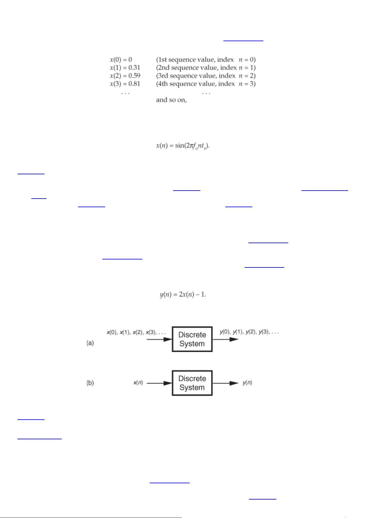
We can reinforce this discrete-time sequence concept by listing those Figure 1-1(b) sampled values as follows:

(1-2)

where n represents the time index integer sequence 0, 1, 2, 3, etc., and t

is some constant time period between

samples. Those sample values can be represented collectively, and concisely, by the discrete-time expression

(1-3)

(Here again, the 2πf

term is an angle measured in radians.) Notice that the index n in

Eq. (1-2) started with a value of 0, instead of 1. There’s nothing sacred about this; the first value of n could just

as well have been 1, but we start the index n at zero out of habit because doing so allows us to describe the

sinewave starting at time zero. The variable x(n) in Eq. (1-3) is read as “the sequence x of n.” Equations (1-1)

and (1-3) describe what are also referred to as time-domain signals because the independent variables, the

continuous time t in Eq. (1-1), and the discrete-time nt

values used in Eq. (1-3) are measures of time.

With this notion of a discrete-time signal in mind, let’s say that a discrete system is a collection of hardware

components, or software routines, that operate on a discrete-time signal sequence. For example, a discrete

system could be a process that gives us a discrete output sequence y(0), y(1), y(2), etc., when a discrete input

sequence of x(0), x(1), x(2), etc., is applied to the system input as shown in Figure 1-2(a). Again, to keep the

notation concise and still keep track of individual elements of the input and output sequences, an abbreviated

notation is used as shown in Figure 1-2(b) where n represents the integer sequence 0, 1, 2, 3, etc. Thus, x(n) and

y(n) are general variables that represent two separate sequences of numbers. Figure 1-2(b) allows us to describe

a system’s output with a simple expression such as

(1-4)

Figure 1-2 With an input applied, a discrete system provides an output: (a) the input and output are sequences

of individual values; (b) input and output using the abbreviated notation of x(n) and y(n).

Illustrating

Eq. (1-4), if x(n) is the five-element sequence x(0) = 1, x(1) = 3, x(2) = 5, x(3) = 7, and x(4) = 9, then y(n) is the

five-element sequence y(0) = 1, y(1) = 5, y(2) = 9, y(3) = 13, and y(4) = 17.

Equation (1-4) is formally called a difference equation. (In this book we won’t be working with differential

equations or partial differential equations. However, we will, now and then, work with partially difficult

equations.)

The fundamental difference between the way time is represented in continuous and discrete systems leads to a

very important difference in how we characterize frequency in continuous and discrete systems. To illustrate,

let’s reconsider the continuous sinewave in Figure 1-1(a). If it represented a voltage at the end of a cable, we

could measure its frequency by applying it to an oscilloscope, a spectrum analyzer, or a frequency counter. We’

d have a problem, however, if we were merely given the list of values from Eq. (1-2) and asked to determine

the frequency of the waveform they represent. We’d graph those discrete values, and, sure enough, we’d

recognize a single sinewave as in Figure 1-1(b). We can say that the sinewave repeats every 20 samples, but

there’s no way to determine the exact sinewave frequency from the discrete sequence values alone. You can

probably see the point we’re leading to here. If we knew the time between samples—the sample period t

—we’

d be able to determine the absolute frequency of the discrete sinewave. Given that the t

sample period is, say,

0.05 milliseconds/sample, the period of the sinewave is

(1-5)

Because the frequency of a sinewave is the reciprocal of its period, we now know that the sinewave’s absolute

frequency is 1/(1 ms), or 1 kHz. On the other hand, if we found that the sample period was, in fact, 2

milliseconds, the discrete samples in

Figure 1-1(b) would represent a sinewave whose period is 40 milliseconds and whose frequency is 25 Hz. The

point here is that when dealing with discrete systems, absolute frequency determination in Hz is dependent on

the sampling frequency

(1-5′)

We’ll be reminded of this dependence throughout the remainder of this book.

In digital signal processing, we often find it necessary to characterize the frequency content of discrete time-

domain signals. When we do so, this frequency representation takes place in what’s called the frequency

domain. By

way of example, let’s say we have a discrete sinewave sequence x

(n) with an arbitrary frequency f

Hz as

shown on the left side of Figure 1-3(a). We can also characterize x

(n) by showing its spectral content, the X

(m) sequence on the right side of Figure 1-3(a), indicating that it has a single spectral component, and no other

frequency content. Although we won’t dwell on it just now, notice that the frequency-domain representations in

Figure 1-3 are themselves discrete.

Figure 1-3 Time- and frequency-domain graphical representations: (a) sinewave of frequency f

; (b) reduced

amplitude sinewave of frequency 2f

; (c) sum of the two sinewaves.

To illustrate our time- and frequency-domain representations further,

Figure 1-3(b) shows another discrete sinewave x

(n), whose peak amplitude is 0.4, with a frequency of 2f

. The

discrete sample values of x

(n) are expressed by the equation

(1-6)

When the two sinewaves, x

(n) and x

(n), are added to produce a new waveform x

sum

(n), its time-domain

equation is

(1-7)

and its time- and frequency-domain representations are those given in

Figure 1-3(c). We interpret the X

sum

(m) frequency-domain depiction, the spectrum, in Figure 1-3(c) to indicate

that x

sum

(n) has a frequency component of f

Hz and a reduced-amplitude frequency component of 2f

Hz.

Notice three things in Figure 1-3. First, time sequences use lowercase variable names like the “x” in x

(n), and

uppercase symbols for frequency-domain variables such as the “X” in X

(m). The term X

(m) is read as “the

spectral sequence X sub one of m.” Second, because the X

(m) frequency-domain representation of the x

(n)

time sequence is itself a sequence (a list of numbers), we use the index “m” to keep track of individual elements

in X

(m). We can list frequency-domain sequences just as we did with the time sequence in Eq. (1-2). For

example, X

sum

(m) is listed as

where the frequency index m is the integer sequence 0, 1, 2, 3, etc. Third, because the x

(n) + x

(n) sinewaves

have a phase shift of zero degrees relative to each other, we didn’t really need to bother depicting this phase

relationship in X

sum

(m) in Figure 1-3(c). In general, however, phase relationships in frequency-domain

sequences are important, and we’ll cover that subject in Chapters 3 and 5.

A key point to keep in mind here is that we now know three equivalent ways to describe a discrete-time

waveform. Mathematically, we can use a time-domain equation like Eq. (1-6). We can also represent a time-

domain waveform graphically as we did on the left side of Figure 1-3, and we can depict its corresponding,

discrete, frequency-domain equivalent as that on the right side of Figure 1-3.

As it turns out, the discrete time-domain signals we’re concerned with are not only quantized in time; their

amplitude values are also quantized. Because we represent all digital quantities with binary numbers, there’s a

limit to the resolution, or granularity, that we have in representing the values of discrete numbers. Although

signal amplitude quantization can be an important consideration—we cover that particular topic in Chapter

12—we won’t worry about it just now.

1.2 Signal Amplitude, Magnitude, Power

Let’s define two important terms that we’ll be using throughout this book: amplitude and magnitude. It’s not

surprising that, to the layman, these terms are typically used interchangeably. When we check our thesaurus,

we find that they are synonymous.

†

In engineering, however, they mean two different things, and we must keep that difference clear in our

discussions. The amplitude of a variable is the measure of how far, and in what direction, that variable differs

from zero. Thus, signal amplitudes can be either positive or negative. The time-domain sequences in Figure 1-3

presented the sample value amplitudes of three different waveforms. Notice how some of the individual

discrete amplitude values were positive and others were negative.

†

Of course, laymen are “other people.” To the engineer, the brain surgeon is the layman. To the brain surgeon, the engineer is the

layman.

The magnitude of a variable, on the other hand, is the measure of how far, regardless of direction, its quantity

differs from zero. So magnitudes are always positive values. Figure 1-4 illustrates how the magnitude of the x

(n) time sequence in Figure 1-3(a) is equal to the amplitude, but with the sign always being positive for the

剩余708页未读，继续阅读

qq_17496741

粉丝: 0

掌握数字信号处理：全新第三版详解与工程实践

深入解析数字信号处理第三版：理论与实践结合

"数字信号处理第四版第10章习题答案解析汇总--计算机方法 英文版

通信工程双语教学：数字信号处理PPT课件概述

understanding digital signal processing

Understanding Digital Signal Processing 3rd

understanding digitalsignal processing朱光明

Understanding Digital Signal Processing - 朱光明

《Understanding Digital Signal Processing》

Understanding Digital Signal Processing 3rd Edition

Understanding Digital Signal Processing, 3rd Edition

最新资源

"数字信号处理第四版第10章习题答案解析汇总--计算机方法英文版