3
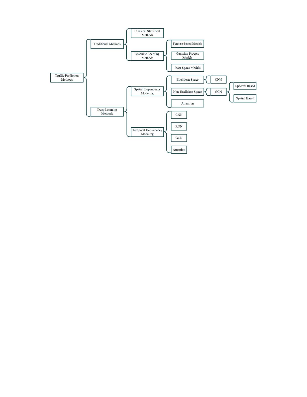
Fig. 2. Categories of traffic prediction methods.
average (ARIMA) [88] and its variants are one of the most
consolidated approaches based on classical statistics and have
been widely applied for traffic prediction problems ( [1], [48],
[58], [64], [73], [82], [88] ). However, these methods are gen-
erally designed for small datasets, and are not suitable to deal
with complex and dynamic time series data. In addition, since
usually only temporal information is considered, the spatial
dependency of traffic data is ignored or barely considered.
Machine learning methods, which can model more complex
data, are broadly divided into three categories: feature-based
models, Gaussian process models and state space models.
Feature-based methods solve traffic prediction problem ( [28],
[47] ) by training a regression model based on human-
engineered traffic features. These methods are simple to
implement and can provide predictions in some practical
situations. Despite this feasibility, feature-based models have
a crucial limitation: the performance of the model depends
heavily on the human-engineered features. Gaussian process
models the inner characteristics of traffic data through different
kernel functions, which need to contain spatial and temporal
correlations simultaneously. Although this kind of method is
proved to be effective and feasible in traffic prediction ( [18],
[56], [71] ), they have higher computational load and storage
pressure, which is not appropriate when a mass of training
samples are available. State space models assume that the
observations are generated by Markovian hidden states. The
advantage of this model is that it can naturally model the
uncertainty of the system and better capture the latent structure
of the spatio-temporal data. However, the overall non-linearity
of these models ( [14], [15], [19], [26], [34], [35], [40], [69],
[75], [79], [98] ) is limited, and most of the time they are not
optimal for modeling complex and dynamic traffic data. Table I
summarizes some recent representative traditional approaches.
III. DEEP LEARNING METHODS
Deep learning models exploit much more features and
complex architectures than the traditional methods, and can
achieve better performance. They have been widely applied
in traffic prediction. In this section, we will review different
deep learning based traffic prediction methods in recent years
according to how they model spatio-temporal correlations.
A. Modeling Spatial Dependency
CNN. A series of studies have applied CNN to capture
spatial correlations in traffic networks from two-dimensional
spatio-temporal traffic data [51]. Since the traffic network is
difficult to be described by 2D matrices, several researches try
to convert the traffic network structure at different times into
images and divide these images into standard grids, with each
grid representing a region. In this way, CNNs can be used to
learn spatial features among different regions.
As shown in Fig. 3, each region is directly connected to its
nearby regions. With a 3×3 window, the neighborhood of each
region is its surrounding eight regions. The positions of these
eight regions indicate an ordering of a region’s neighbors. A
filter is then applied to this 3× 3 patch by taking the weighted
average of the central region and its neighbors across each
channel. Due to the specific ordering of neighboring regions,
the trainable weights are able to be shared across different
locations.
In the division of traffic road network structure, there are
many definitions of positions according to different granularity
and semantic meanings. [102] divided a city into I J grid maps
based on the longitude and latitude where a grid representd a
region. Then, a CNN was applied to extract the spatial corre-
lation between different regions for traffic flow prediction.


