粒子滤波器详解：非线性/非高斯贝叶斯跟踪教程

需积分: 10 161 浏览量更新于2024-07-23 1 收藏 355KB PDF 举报

粒子滤波器教程在本文档中，作者Sanjeev Arulampalam、Simon Maskell、Neil Gordon和Tim Clapp为我们提供了一篇关于在线非线性/非高斯贝叶斯跟踪的粒子滤波器教程。随着技术的发展，许多应用领域越来越需要考虑系统的非线性和非高斯特性，以更准确地模拟物理过程。实时处理数据变得至关重要，这既是为了减少存储成本，也是为了快速适应不断变化的信号特征。粒子滤波器是一种基于蒙特卡洛方法的统计学工具，其核心思想是通过离散的概率密度函数（即“粒子”）来表示系统状态。与传统的卡尔曼滤波方法相比，粒子滤波器具有更大的灵活性，能够处理非线性和非高斯性的动态问题。它在状态空间模型中非常适用，允许在序列决策过程中进行概率分布的估计和更新。该教程首先介绍了最优和次优的贝叶斯算法，这些算法旨在解决非线性/非高斯跟踪问题。其中，重点放在了粒子滤波器的不同变种上，如： 1. **SIR (Sequential Importance Resampling)**：这种方法通过根据粒子的重要性采样，对粒子集合进行重新采样，以保持整体分布的多样性，防止过早衰减。 2. **ASIR (Adaptive SIR)**：ASIR是在SIR的基础上进一步优化，通过自适应调整采样策略，以提高算法的效率和精度。 3. **RPF (Resampling Particle Filter)**：粒子滤波器的一个关键步骤是重采样，RPF方法提供了多种策略，如基于阈值的重采样，旨在在粒子稀疏度达到一定程度时平衡计算效率和准确性。论文详细讨论了这些方法的原理、应用场景和它们在实际问题中的优势和局限性。此外，还涉及到了如何选择合适的粒子数量、如何处理观测噪声以及如何处理系统模型中的不确定性等问题。通过这篇教程，读者可以深入了解粒子滤波器的理论基础和实践应用，对于从事在线非线性/非高斯环境下的目标跟踪、机器人导航、信号处理等领域的工作来说，是一份非常有价值的参考资料。

176 IEEE TRANSACTIONS ON SIGNAL PROCESSING, VOL. 50, NO. 2, FEBRUARY 2002

where

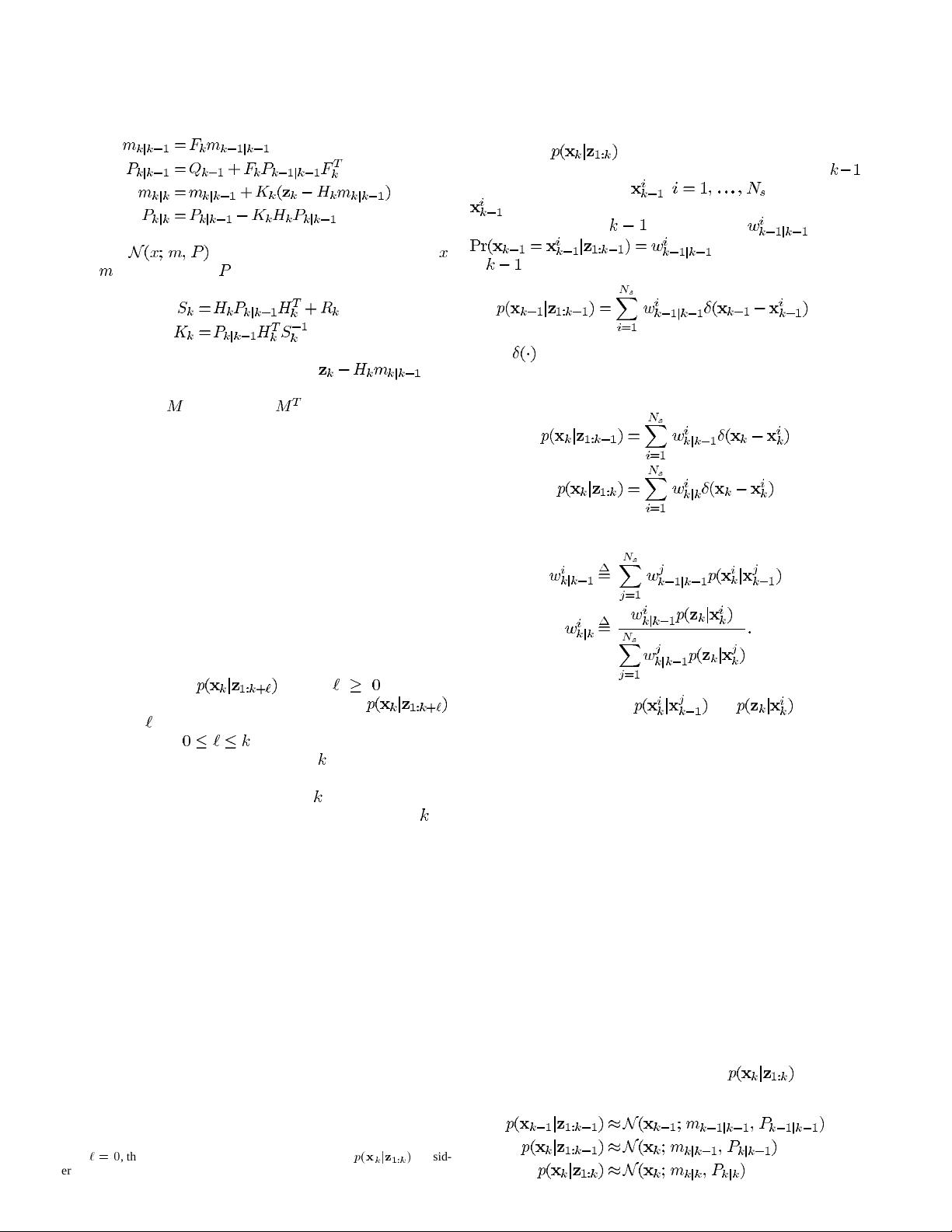
(11)

(12)

(13)

(14)

and where

is a Gaussian density with argument ,

mean

, and covariance , and

(15)

(16)

are the covariance of the innovation term

, and

the Kalman gain, respectively. In the above equations, the trans-

pose of a matrix

is denoted by .

This is the optimal solution to the tracking problem—if the

(highly restrictive) assumptions hold. The implication is that no

algorithm can ever do better than a Kalman filter in this linear

Gaussian environment. It should be noted that it is possible to

derive the same results using a least squares (LS) argument [22].

All the distributions are then described by their means and co-

variances, and the algorithm remains unaltered, but are not con-

strained to be Gaussian. Assuming the means and covariances

to be unbiased and consistent, the filter then optimally derives

the mean and covariance of the posterior. However, this poste-

rior is not necessarily Gaussian, and therefore, if optimality is

the ability of an algorithm to calculate the posterior, the filter is

then not certain to be optimal.

Similarly, if smoothed estimates of the states are required,

that is, estimates of

, where ,

then the

Kalman smoother is the optimal estimator of

This holds if

is fixed (fixed-lag smoothing, if a batch of data

are considered and

(fixed-interval smoothing), or if

the state at a particular time is of interest

is fixed (fixed-point

smoothing). The problem of calculating smoothed densities is

of interest because the densities at time

are then conditional

not only on measurements up to and including time index

but

also on future measurements. Since there is more information

on which to base the estimation, these smoothed densities are

typically tighter than the filtered densities.

Although this is true, there is an algorithmic issue that should

be highlighted here. It is possible to formulate a backward-time

Kalman filter that recurses through the data sequence from the

final data to the first and then combines the estimates from the

forward and backward passes to obtain overall smoothed es-

timates [20]. A different formulation implicitly calculates the

backward-time state estimates and covariances, recursively esti-

mating the smoothed quantities [38]. Both techniques are prone

to having to calculate matrix inverses that do not necessarily

exist. Instead, it is preferable to propagate different quantities

using an information filter when carrying out the backward-time

recursion [4].

, then the problem reduces to the estimation of

(

)

consid-

ered up to this point.

B. Grid-Based Methods

Grid-based methods provide the optimal recursion of the fil-

tered density

if the state space is discrete and consists

of a finite number of states. Suppose the state space at time

consists of discrete states , . For each state

, let the conditional probability of that state, given mea-

surements up to time

be denoted by , that is,

. Then, the posterior pdf

can be written as

(17)

where

is the Dirac delta measure. Substitution of (17) into

(3) and (4) yields the prediction and update equations, respec-

tively

(18)

(19)

where

(20)

(21)

The above assumes that

and are known

butdoes not constrain the particular form of these discrete densi-

ties. Again, this is the optimal solution if the assumptions made

hold.

IV. S

UBOPTIMAL ALGORITHMS

In many situations of interest, the assumptions made above

do not hold. The Kalman filter and grid-based methods cannot,

therefore, be used as described—approximations are necessary.

In this section, we consider three approximate nonlinear

Bayesian filters:

a) extended Kalman filter (EKF);

b) approximate grid-based methods;

c) particle filters.

A. Extended Kalman Filter

If (1) and (2) cannot be rewritten in the form of (6) and (7)

because the functions are nonlinear, then a local linearization of

the equations may be a sufficient description of the nonlinearity.

The EKF is based on this approximation.

is approx-

imated by a Gaussian

(22)

(23)

(24)

剩余14页未读，继续阅读

「已注销」

粉丝: 0
资源: 1

粒子滤波器详解：非线性/非高斯贝叶斯跟踪教程

Durrant Whyte Bailey SLAM-tutorial-I

PF_Tutorial_Crack.rar_Paris公式_paris_寿命_疲劳寿命计算_粒子滤波

pmh-tutorial：该教程的源代码和数据：“粒子Metropolis-Hastings入门，用于非线性模型的推理”

广东工业大学22级物联网工程概率论复习资料

Image_226679847094279.jpg

java项目，课程设计-ssm留学生交流互动论坛网站.zip

java超市销售管理系统源码 超市综合管理系统源码数据库 MySQL源码类型 WebForm

【小程序毕业设计】基于微信小程序的夏津县汽车站购票系统设计与实现源码（完整前后端+mysql+说明文档）.zip

实验四 PL/SQL编程

通过Python，Tkinter，文本文件，Openpyxl 实现【图书馆管理系统实现技术】

最新资源

java超市销售管理系统源码超市综合管理系统源码数据库 MySQL源码类型 WebForm