基于噪声模型的v-SVR:风速预测中的有效预测技术
下载需积分: 15 | PDF格式 | 996KB |
更新于2024-08-26
| 132 浏览量 | 举报
本文主要探讨了基于噪声模型的v-支持向量回归(Noise Model Based ν-Support Vector Regression, N-SVR)及其在短期风速预测中的应用。支持向量回归(SVR)作为一种强大的机器学习工具,其核心思想是通过构建最优超平面来实现对复杂非线性关系的学习。然而,现实世界中的许多数据集可能存在非高斯噪声,如β分布或拉普拉斯分布,这可能会影响传统的高斯噪声假设下的回归性能。
作者首先指出,现有的SVR技术在处理这类非高斯噪声时可能存在局限性,因为它们依赖于高斯分布的假设。为了克服这个问题,他们提出了一种新的方法,即N-SVR,这是一种能够适应一般噪声模型的回归框架。N-SVR的核心是引入了一般损失函数,这个函数考虑了不同类型的噪声分布,从而提高了模型的鲁棒性。
在N-SVR的实现中,作者利用了增强拉格朗日乘子法来解决不等式约束问题,这是一个优化问题的关键步骤。这种方法允许模型同时处理线性和非线性决策边界,以及噪声数据带来的复杂性。通过这种方式,N-SVR能够在保持模型简洁性和泛化能力的同时,更准确地捕获实际数据中的潜在规律。
接下来,作者通过在人工数据集、UCI数据集以及实际的短期风速预测问题上进行数值实验,验证了N-SVR的有效性和优越性。风速预测是一个典型的应用场景,其中准确性至关重要,因为风能是一种可再生能源,其产量受到诸多因素的影响,包括风速的短期变化。N-SVR在处理这类具有非高斯噪声的风速数据时,显示出比传统方法更好的预测性能。
总结来说,本文贡献了一个新颖的噪声模型支持向量回归技术,它不仅扩展了SVR的应用范围,而且在实际问题如风速预测中取得了显著的预测效果。这一研究对于提升预测模型的稳健性和准确性,特别是在处理非高斯噪声的数据集时,具有重要的理论价值和实践意义。
Q. Hu et al. / Neural Networks 57 (2014) 1–11 3
we derive a general loss function and construct ν-support vector
regression machines for a general noise model.
Finally, we design a technique to find the optimal solution to the
corresponding regression tasks. While there are a large number of
implementations of SVR algorithms in the past years, we introduce
the Augmented Lagrange Multiplier (ALM) method, presented in
Section 4. If the task is non-differentiable or discontinuous, the
sub-gradient descent method can be used (Ma, 2010), and if there
are very large scale of samples, SMO can also be used (Shevade,
Keerthi, Bhattacharyya, & Murthy, 2000).
The main contributions of our work are listed as follows: (1) we
derive the optimal loss functions for different error models by the
use of Bayesian approach and optimization theory; (2) we develop
the uniform ν-support vector regression model for the general
noise with inequality constraints (N-SVR); (3) the Augmented
Lagrange Multiplier method is applied to solve N-SVR, which
guarantees the stability and validity of the solution in N-SVR;
(4) we utilize N-SVR to short-term wind speed prediction and show
the effectiveness of the proposed model in practical applications.
This paper is organized as follows: in Section 2 we derive the
optimal loss function corresponding to a noise model by using
the Bayesian approach; in Section 3 we describe the proposed
ν-support vector regression technique for general noise model
(N-SVR); in Section 4 we give the solution and algorithm design
of N-SVR; numerical experiments are conducted on artificial data
sets, UCI data and short-term wind speed prediction in Sections 5
and 6; finally, we conclude the work in Section 7.
2. Bayesian approach to the general loss function
Given a set of noisy training samples D
l
, we require to estimate
an unknown function f (x). Following Chu, Keerthi, and Ong (2004);
Girosi (1991); Klaus-Robert and Sebastian (2001); Pontil et al.
(1998), the general approach is to minimize
H[f ] =
l
i=1
c(ξ
i
) + λ · Φ[f ], (7)
where c(ξ
i
) = c(y
i
−f (x
i
)) is a loss function, λ is a positive number
and Φ[f ] is a smoothness functional.
We assume the noise is additive
y
i
= f (x
i
) + ξ
i
, i = 1, 2, . . . , l, (8)
where ξ
i
is random, independent, identical probability distribu-
tions (i.i.d.) with P(ξ
i
) of variance σ and mean µ. We want to es-
timate the function f (x) with the set of data D
f
⊆ D
l
. We take a
probabilistic approach, and regard the function f as the realization
of a random field with a known prior probability distribution. We
are interested in maximizing the posteriori probability of f given
the data D
f
, namely P[f |D
f
], which can be written as
P[f |D
f
] ∝ P[D
f
|f ] · P[f ], (9)
where P[D
f
|f ] is the conditional probability of the data D
f
given
the function f and P[f ] is a priori probability of the random field
f , which is often written as P[f ] ∝ exp(−λ · Φ[f ]), where Φ[f ]
is a smoothness functional. The probability P[D
f
|f ] is essentially a
model of the noise, and if the noise is additive, as in Eq. (8) and i.i.d.
with probability distribution P(ξ
i
), it can be written as
P[D
f
|f ] =
l
i=1
P(ξ
i
). (10)
Substituting P[f ] and Eq. (10) in (9), we see that the function
that maximizes the posterior probability of f is the one which
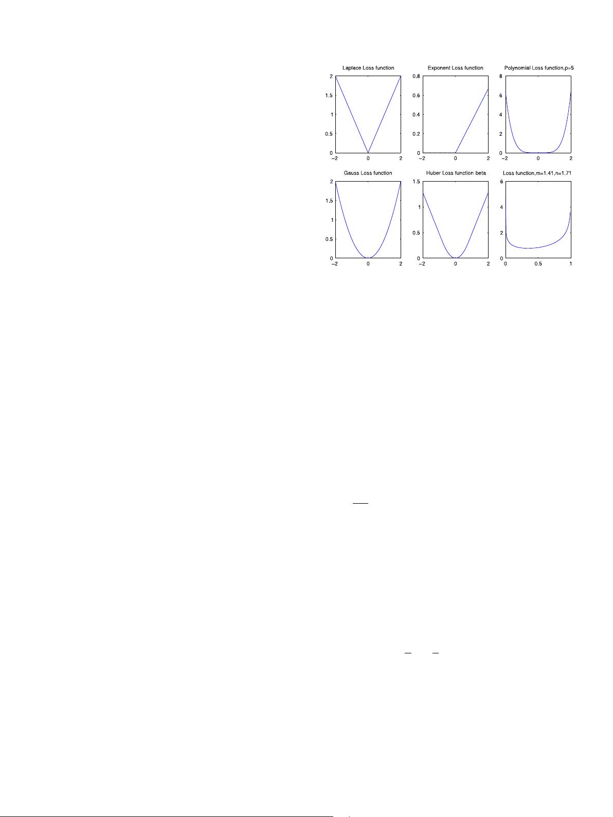
Fig. 2. Loss function of the corresponding noise model.
minimizes the following functional
H[f ] = −
l
i=1
log[P(y
i
− f (x
i
)) · e
−λ·Φ[f ]
]
= −
l
i=1
log P(y
i
− f (x
i
)) + λ · Φ[f ]. (11)
This functional is of the same form as Eq. (7) (Girosi, 1991; Pontil
et al., 1998). By Eqs. (7) and (11), the optimal loss function in a
maximum likelihood sense is
c(x, y, f (x)) = −log p(y − f (x)), (12)
i.e. the loss function c(ξ ) is the log-likelihood of the noise.
We assume that the noise in Eq. (8) is Gaussian, with zero mean
and variance σ . By Eq. (12), the loss function corresponding to
Gaussian-noise is
c(ξ
i
) =
1
2σ
2
(y
i
− f (x
i
))
2
. (13)
If the noise in Eq. (8) is beta, with mean µ ∈ (0, 1) and variance
σ , get m = (1−µ)·µ
2
/σ
2
−µ, n = ((1−µ)/µ)·m (m > 1, n > 1),
and h = Γ (m + n)/(Γ (m) · Γ (n)) is the normalization factor
(Bofinger et al., 2002). By Eq. (12), the loss function corresponding
to beta-noise is
c(ξ
i
) = (1 − m) log(ξ
i
) + (1 − n) log(1 − ξ
i
), (14)
where parameters m > 1, n > 1.
And if the noise in Eq. (8) is Weibull, with parameters θ and k.
By Eq. (12), the loss function should be
c(ξ
i
) =
(1 − k) log
ξ
i
θ
+
ξ
i
θ
k
, if ξ
i
≥ 0,
0, otherwise.
(15)
The loss functions and their corresponding probability density
functions (PDF) of the noise models used in regression problems
are listed in Table 1 and shown in Fig. 2.
3. Noise model based ν-support vector regression
Given samples D
l
, we construct a linear regression function
f (x) = ω
T
· x + b. In order to deal with nonlinear functions the
剩余10页未读,继续阅读
相关推荐


weixin_38698367
- 粉丝: 4
 我的内容管理
展开
我的内容管理
展开


最新资源
- C#实现Console与Form界面加法运算教程
- Neuroph 2.9:轻量级Java神经网络框架及GUI应用
- 流星运行时Fibers模块实现同步异步编程
- IOS中TableView箭头颜色更改教程及图片示例
- Springboot文件上传功能实现与端口路径配置
- TorrSE 2.0.2_mod_signed_zipalign:磁力链接爬虫软件
- 微信小程序开发实战:辣椒忍者源码解析
- QuadMinds通知扩展插件:桌面事件即时通知
- QQPhoneManager压缩包文件解析与管理技巧
- 掌握数据库活动管理:JavaScript开发者的必备指南
- 易语言实现倍数判断功能的源码分析
- 掌握在线PDF预览技术:前端至后端完整实现
- 易特商业销售管理系统:全面解决方案与高效管理
- IOS源码:Scream.swift封装target和selector
- 全面兼容主流浏览器的纯JavaScript日历
- 探索动态广播在页面间通信的实现方法
